Warning: package 'tidyr' was built under R version 4.2.3
Warning: package 'readr' was built under R version 4.2.3
Warning: package 'dplyr' was built under R version 4.2.3
Warning: package 'stringr' was built under R version 4.2.3
── Attaching core tidyverse packages ──────────────────────── tidyverse 2.0.0 ──
✔ dplyr     1.1.4     ✔ readr     2.1.5
✔ forcats   1.0.0     ✔ stringr   1.5.1
✔ ggplot2   3.5.2     ✔ tibble    3.2.1
✔ lubridate 1.9.4     ✔ tidyr     1.3.1
✔ purrr     1.0.2
── Conflicts ────────────────────────────────────────── tidyverse_conflicts() ──
✖ dplyr::filter() masks stats::filter()
✖ dplyr::lag()    masks stats::lag()
ℹ Use the conflicted package (<http://conflicted.r-lib.org/>) to force all conflicts to become errors
library(lubridate)library(brms)
Warning: package 'brms' was built under R version 4.2.3
Loading required package: Rcpp
Loading 'brms' package (version 2.21.0). Useful instructions
can be found by typing help('brms'). A more detailed introduction
to the package is available through vignette('brms_overview').

Attaching package: 'brms'

The following object is masked from 'package:stats':

    ar
Warning: package 'bayestestR' was built under R version 4.2.3
library(marginaleffects)
Warning: package 'marginaleffects' was built under R version 4.2.3
library(rstan)
Warning: package 'rstan' was built under R version 4.2.3
Loading required package: StanHeaders

rstan version 2.32.6 (Stan version 2.32.2)

For execution on a local, multicore CPU with excess RAM we recommend calling
options(mc.cores = parallel::detectCores()).
To avoid recompilation of unchanged Stan programs, we recommend calling
rstan_options(auto_write = TRUE)
For within-chain threading using `reduce_sum()` or `map_rect()` Stan functions,
change `threads_per_chain` option:
rstan_options(threads_per_chain = 1)


Attaching package: 'rstan'

The following object is masked from 'package:tidyr':

    extract
library(flowchart)library("devtools")
Loading required package: usethis
library(rcmswe)# Set gtsummart themetheme_gtsummary_compact()
New names:
Rows: 109107 Columns: 127
── Column specification
──────────────────────────────────────────────────────── Delimiter: ";" chr
(18): DX_GROUP, hospital_name_receiving, sir_icu_name, sir_hospital_typ... dbl
(91): ...1, VtfId_LopNr, TERTIARY_HADM_ID, LopNr, SIR_PAR_OFFSET, SIR_P... lgl
(8): daylight, hems_minima_sending, hems_minima_window, daylight_recei... dttm
(9): sir_adm_time, sir_dsc_time, sir_adm_time_UTC, sir_dsc_time_UTC, w... date
(1): DODSDAT_ROUND_UP
ℹ Use `spec()` to retrieve the full column specification for this data. ℹ
Specify the column types or set `show_col_types = FALSE` to quiet this message.
• `` -> `...1`
# Prune datad_pruned <- d %>%filter(sir_dsc_time >="2019-10-01"& sir_dsc_time <="2024-05-15") %>%# 2019-10-01 -- 2024-05-15filter(!is.na(TERTIARY_HADM_ID)) %>%# Keep only rows with a tertiary HADM matchfilter(sir_total_time <=720) %>%# Keep only rows with a primary ICU stay 12 hours or shorterfilter(SIR_PAR_OFFSET_TIGHT %in% (c(-1,0,1))) %>%# Keep only rows with a recent PAR admitfilter(road_distance >=45) %>%# Keep only rows with transfers 45 km or longerfilter(DX_GROUP %in%c("ASAH", "ICH", "AIS", "TBI")) %>%#Keep only admits with ASAH, ICH, AIS or TBIfilter(min_rank(DX_RANK) ==1, .by = VtfId_LopNr) %>%# Within each unique VtfId_LopNr, keep only the lowest ranking diagnostic PAR admitslice_max(sir_dsc_time, by = LopNr, n =1, with_ties =FALSE) # This gives the latest date by default (if ties, may give more than one)
In [2]:
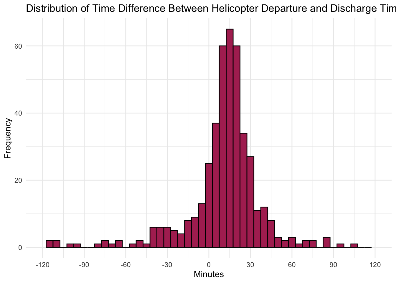
# Create transfers plotdsc_time <-ymd_hms(d_pruned$sir_dsc_time_UTC, tz="UTC")out_time <-ymd_hms(d_pruned$UTC_out_sending_hems, tz="UTC")timediff_minutes <-data.frame((out_time - dsc_time) /60)names(timediff_minutes) <-c("SIR_discharge_time_relative_helicopter_out_time")plot_timediff <-ggplot(timediff_minutes, aes(x = SIR_discharge_time_relative_helicopter_out_time)) +geom_histogram(binwidth =5, fill ="maroon", color ="black") +labs(title ="Distribution of Time Difference Between Helicopter Departure and Discharge Time",x ="Minutes", y ="Frequency") +scale_x_continuous(limits =c(-120, 120),breaks =c(-120, -90, -60, -30, 0, 30, 60, 90, 120) ) +theme_minimal()
In [3]:
plot_timediff
Warning: Removed 1381 rows containing non-finite outside the scale range
(`stat_bin()`).
Warning: Removed 2 rows containing missing values or values outside the scale range
(`geom_bar()`).
Distribution of time differences between helicopter departure from the sending hospital and the recorded ICU discharge time. Positive values indicate that the helicopter departed after ICU discharge; negative values indicate departure before the documented discharge time. The ±120-minute window was used to define a matched helicopter transfer as the tails of the distribution reached a uniform plateau.
(fig-timediff?) shows the distribution of time differences between ICU discharge and matched flight departures. Transfers without a corresponding flight in the ADS-B dataset were classified as using another transport modality.