Back to Article
Causal Effects of Helicopter Emergency Medical Services Research -in Interfacility Transfers to Neuro ICUs - A Study Using Swedish National Registries (2019–2024)
Download Source

Causal Effects of Helicopter Emergency Medical Services Research -in Interfacility Transfers to Neuro ICUs - A Study Using Swedish National Registries (2019–2024)

Authors
Affiliations

Johan Olsson

Department of Pediatric Perioperative Medicine and Intensive Care, ECMO Centre Karolinska, Karolinska University Hospital, Stockholm, Sweden; Department of Physiology and Pharmacology, Karolinska Institutet, Stockholm, Sweden.

Ryan Falck-Jones

Department of Perioperative Medicine and Intensive Care, Karolinska University Hospital, Stockholm, Sweden; Department of Physiology and Pharmacology, Karolinska Institutet, Stockholm, Sweden.

Anders Holst

School of Electrical Engineering and Computer Science, KTH Royal Institute of Technology, Stockholm, Sweden.

Cecilia Åkerlund

Department of Perioperative Medicine and Intensive Care, Karolinska University Hospital, Stockholm, Sweden; Department of Physiology and Pharmacology, Karolinska Institutet, Stockholm, Sweden.

Logan Froese

Department of Clinical Neuroscience, Karolinska Institutet, Stockholm, Sweden.

Linn Hallqvist

Department of Perioperative Medicine and Intensive Care, Karolinska University Hospital, Stockholm, Sweden; Department of Physiology and Pharmacology, Karolinska Institutet, Stockholm, Sweden.

Published

July 8, 2025

Keywords

Neurocritical care, Neurointensive care, Intensive care, NSICU, Neurosurgical intensive care, Interfacility transfer, Causal inference, Instrumental variable analysis, HEMS, Patient transfer

In [1]:
# Load dependencies 
library(tidyverse)
Warning: package 'tidyr' was built under R version 4.2.3
Warning: package 'readr' was built under R version 4.2.3
Warning: package 'dplyr' was built under R version 4.2.3
Warning: package 'stringr' was built under R version 4.2.3
── Attaching core tidyverse packages ──────────────────────── tidyverse 2.0.0 ──
✔ dplyr     1.1.4     ✔ readr     2.1.5
✔ forcats   1.0.0     ✔ stringr   1.5.1
✔ ggplot2   3.5.2     ✔ tibble    3.2.1
✔ lubridate 1.9.4     ✔ tidyr     1.3.1
✔ purrr     1.0.2     
── Conflicts ────────────────────────────────────────── tidyverse_conflicts() ──
✖ dplyr::filter() masks stats::filter()
✖ dplyr::lag()    masks stats::lag()
ℹ Use the conflicted package (<http://conflicted.r-lib.org/>) to force all conflicts to become errors
library(lubridate)
library(brms)
Warning: package 'brms' was built under R version 4.2.3
Loading required package: Rcpp
Loading 'brms' package (version 2.21.0). Useful instructions
can be found by typing help('brms'). A more detailed introduction
to the package is available through vignette('brms_overview').

Attaching package: 'brms'

The following object is masked from 'package:stats':

    ar
library(DBI)
library(RSQLite)
library(flowchart)
library(gtsummary)
library(ggplot2)
library(bayestestR)
Warning: package 'bayestestR' was built under R version 4.2.3
library(marginaleffects)
Warning: package 'marginaleffects' was built under R version 4.2.3
library(rstan)
Warning: package 'rstan' was built under R version 4.2.3
Loading required package: StanHeaders

rstan version 2.32.6 (Stan version 2.32.2)

For execution on a local, multicore CPU with excess RAM we recommend calling
options(mc.cores = parallel::detectCores()).
To avoid recompilation of unchanged Stan programs, we recommend calling
rstan_options(auto_write = TRUE)
For within-chain threading using `reduce_sum()` or `map_rect()` Stan functions,
change `threads_per_chain` option:
rstan_options(threads_per_chain = 1)


Attaching package: 'rstan'

The following object is masked from 'package:tidyr':

    extract
library(flowchart)
library("devtools")
Loading required package: usethis
library(rcmswe)
library(NatParksPalettes)
library(showtext)
Warning: package 'showtext' was built under R version 4.2.3
Loading required package: sysfonts
Warning: package 'sysfonts' was built under R version 4.2.3
Loading required package: showtextdb
font_add_google("Noto Sans", "Noto Sans")  # Downloads from Google Fonts
showtext_auto()

# Set gtsummart theme
theme_gtsummary_compact()
Setting theme `Compact`
# Load data
d <- read_delim(file = "~/PhD/nsicu-transfers/data/pre-processed-data/patient-df-2025-05-25 22:12:51.563534.csv", delim = ";")[ , -1]
New names:
Rows: 109107 Columns: 127
── Column specification
──────────────────────────────────────────────────────── Delimiter: ";" chr
(18): DX_GROUP, hospital_name_receiving, sir_icu_name, sir_hospital_typ... dbl
(91): ...1, VtfId_LopNr, TERTIARY_HADM_ID, LopNr, SIR_PAR_OFFSET, SIR_P... lgl
(8): daylight, hems_minima_sending, hems_minima_window, daylight_recei... dttm
(9): sir_adm_time, sir_dsc_time, sir_adm_time_UTC, sir_dsc_time_UTC, w... date
(1): DODSDAT_ROUND_UP
ℹ Use `spec()` to retrieve the full column specification for this data. ℹ
Specify the column types or set `show_col_types = FALSE` to quiet this message.
• `` -> `...1`
 #add comorb per Ryan
#lopnr_date <- d %>% select(c("LopNr", "sir_adm_time_UTC"))
#lopnr_date$sir_adm_time_UTC = lopnr_date$sir_adm_time_UTC - as.difftime(7, units = "days")
#comorb <- rcmswe:::extract_comorbs(search_df = lopnr_date, sqlite_path = "~/PhD/datauttag/2025/db_2025.sqlite", LMED=FALSE)
#d <- d %>% left_join(comorb) %>% mutate(CCIunw = replace_na(CCIunw, 0)) %>% mutate(CCIw = replace_na(CCIw, 0))

#d <- d %>%
#  mutate(
#    CCIunw_abr = case_when(
#      CCIunw %in% c(0, 1) ~ "0-1",
#      CCIunw %in% c(2, 3) ~ "2-3",
#      CCIunw >= 4 ~ "≥4"
#    ),
#    CCIunw_abr = factor(CCIunw_abr, levels = c("0-1", "2-3", "≥4"))
#  )

# Prune data
d_pruned <- d %>%
  filter(sir_dsc_time >= "2019-10-01" & sir_dsc_time <= "2024-05-15") %>% # 2019-10-01 -- 2024-05-15
  filter(!is.na(TERTIARY_HADM_ID)) %>%                  # Keep only rows with a tertiary HADM match
  filter(sir_total_time <= 720) %>%                     # Keep only rows with a primary ICU stay 12 hours or shorter
  filter(SIR_PAR_OFFSET_TIGHT %in% (c(-1,0,1))) %>%     # Keep only rows with a recent PAR admit
  filter(road_distance >= 45) %>%                       # Keep only rows with transfers 45 km or longer
  filter(DX_GROUP %in% c("ASAH", "ICH", "AIS", "TBI")) %>% #Keep only admits with ASAH, ICH, AIS or TBI
  filter(min_rank(DX_RANK) == 1, .by = VtfId_LopNr) %>% # Within each unique VtfId_LopNr, keep only the lowest ranking diagnostic PAR admit
  slice_max(sir_dsc_time, by = LopNr, n = 1, with_ties = FALSE) # This gives the latest date by default (if ties, may give more than one)

heavy_users <- d_pruned %>% group_by(formatted_icu_name) %>%
  summarise(
    proportion_hems_ift = mean(hems_ift == TRUE, na.rm = TRUE),
    n = n()
  ) %>%
  filter(proportion_hems_ift >= 0.1) %>%
  select(formatted_icu_name) %>%
  unique()

light_users <- d_pruned %>% group_by(formatted_icu_name) %>%
  summarise(
    proportion_hems_ift = mean(hems_ift == TRUE, na.rm = TRUE),
    n = n()
  ) %>%
  filter(proportion_hems_ift < 0.1) %>%
  select(formatted_icu_name) %>%
  unique()
In [2]:
# Create transfers plot

dsc_time <- ymd_hms(d_pruned$sir_dsc_time_UTC, tz="UTC")
out_time <-  ymd_hms(d_pruned$UTC_out_sending_hems, tz="UTC")
timediff_minutes <- data.frame((out_time - dsc_time) / 60)
names(timediff_minutes) <- c("SIR_discharge_time_relative_helicopter_out_time")

plot_timediff <- ggplot(timediff_minutes, aes(x = SIR_discharge_time_relative_helicopter_out_time)) +
  geom_histogram(binwidth = 5, fill = "maroon", color = "black") +
  labs(title = "Distribution of Time Difference Between Helicopter Departure and Discharge Time",
       x = "Minutes", y = "Frequency") +
  scale_x_continuous(
    limits = c(-120, 120),
    breaks = c(-120, -90, -60, -30, 0, 30, 60, 90, 120)
  ) +
  theme_minimal()
In [3]:
# Check IV relevance in uv model

m.modality.univ <- d_pruned %>%
  filter(!formatted_icu_name %in% light_users$formatted_icu_name) %>%
  mutate(z_SAPS_score_minus_age_and_gcs = scale(SAPS_score_minus_age_and_gcs)) %>%
  mutate(z_age = scale(age)) %>%
  mutate(
    DX_GROUP = forcats::fct_relabel(DX_GROUP, ~ gsub("_", "-", .)),
    sir_consciousness_level = forcats::fct_relabel(sir_consciousness_level, ~ gsub("≤", "le", .))  # or use ASCII-safe levels
  ) %>% brm(
  formula = hems_ift ~ hems_minima_both,
  data = .,
  family = bernoulli(),
  cores = 4,
  chains = 4
)
Warning: Rows containing NAs were excluded from the model.
Compiling Stan program...
Trying to compile a simple C file
Running /Library/Frameworks/R.framework/Resources/bin/R CMD SHLIB foo.c
clang -arch arm64 -I"/Library/Frameworks/R.framework/Resources/include" -DNDEBUG   -I"/Library/Frameworks/R.framework/Versions/4.2-arm64/Resources/library/Rcpp/include/"  -I"/Library/Frameworks/R.framework/Versions/4.2-arm64/Resources/library/RcppEigen/include/"  -I"/Library/Frameworks/R.framework/Versions/4.2-arm64/Resources/library/RcppEigen/include/unsupported"  -I"/Library/Frameworks/R.framework/Versions/4.2-arm64/Resources/library/BH/include" -I"/Library/Frameworks/R.framework/Versions/4.2-arm64/Resources/library/StanHeaders/include/src/"  -I"/Library/Frameworks/R.framework/Versions/4.2-arm64/Resources/library/StanHeaders/include/"  -I"/Library/Frameworks/R.framework/Versions/4.2-arm64/Resources/library/RcppParallel/include/"  -I"/Library/Frameworks/R.framework/Versions/4.2-arm64/Resources/library/rstan/include" -DEIGEN_NO_DEBUG  -DBOOST_DISABLE_ASSERTS  -DBOOST_PENDING_INTEGER_LOG2_HPP  -DSTAN_THREADS  -DUSE_STANC3 -DSTRICT_R_HEADERS  -DBOOST_PHOENIX_NO_VARIADIC_EXPRESSION  -D_HAS_AUTO_PTR_ETC=0  -include '/Library/Frameworks/R.framework/Versions/4.2-arm64/Resources/library/StanHeaders/include/stan/math/prim/fun/Eigen.hpp'  -D_REENTRANT -DRCPP_PARALLEL_USE_TBB=1   -I/opt/R/arm64/include   -fPIC  -falign-functions=64 -Wall -g -O2  -c foo.c -o foo.o
In file included from <built-in>:1:
In file included from /Library/Frameworks/R.framework/Versions/4.2-arm64/Resources/library/StanHeaders/include/stan/math/prim/fun/Eigen.hpp:22:
In file included from /Library/Frameworks/R.framework/Versions/4.2-arm64/Resources/library/RcppEigen/include/Eigen/Dense:1:
In file included from /Library/Frameworks/R.framework/Versions/4.2-arm64/Resources/library/RcppEigen/include/Eigen/Core:19:
/Library/Frameworks/R.framework/Versions/4.2-arm64/Resources/library/RcppEigen/include/Eigen/src/Core/util/Macros.h:679:10: fatal error: 'cmath' file not found
  679 | #include <cmath>
      |          ^~~~~~~
1 error generated.
make: *** [foo.o] Error 1
Start sampling
m.modality.univ_exp_vals <- summary(m.modality.univ)$fixed %>%
  slice(2) %>%
  select("Estimate", "l-95% CI", "u-95% CI") %>%
  unlist() %>%
  exp()
In [4]:
# Check iv model exclusion restriction assumtion

m.weather.mort <- d_pruned %>% 
  filter(formatted_icu_name %in% light_users$formatted_icu_name) %>%
  brm(
    formula = MORTALITY_30D ~ hems_minima_both,
    data = .,
    family = bernoulli(),
    cores = 4,
    chains = 4
  )
Warning: Rows containing NAs were excluded from the model.
Compiling Stan program...
Trying to compile a simple C file
Running /Library/Frameworks/R.framework/Resources/bin/R CMD SHLIB foo.c
clang -arch arm64 -I"/Library/Frameworks/R.framework/Resources/include" -DNDEBUG   -I"/Library/Frameworks/R.framework/Versions/4.2-arm64/Resources/library/Rcpp/include/"  -I"/Library/Frameworks/R.framework/Versions/4.2-arm64/Resources/library/RcppEigen/include/"  -I"/Library/Frameworks/R.framework/Versions/4.2-arm64/Resources/library/RcppEigen/include/unsupported"  -I"/Library/Frameworks/R.framework/Versions/4.2-arm64/Resources/library/BH/include" -I"/Library/Frameworks/R.framework/Versions/4.2-arm64/Resources/library/StanHeaders/include/src/"  -I"/Library/Frameworks/R.framework/Versions/4.2-arm64/Resources/library/StanHeaders/include/"  -I"/Library/Frameworks/R.framework/Versions/4.2-arm64/Resources/library/RcppParallel/include/"  -I"/Library/Frameworks/R.framework/Versions/4.2-arm64/Resources/library/rstan/include" -DEIGEN_NO_DEBUG  -DBOOST_DISABLE_ASSERTS  -DBOOST_PENDING_INTEGER_LOG2_HPP  -DSTAN_THREADS  -DUSE_STANC3 -DSTRICT_R_HEADERS  -DBOOST_PHOENIX_NO_VARIADIC_EXPRESSION  -D_HAS_AUTO_PTR_ETC=0  -include '/Library/Frameworks/R.framework/Versions/4.2-arm64/Resources/library/StanHeaders/include/stan/math/prim/fun/Eigen.hpp'  -D_REENTRANT -DRCPP_PARALLEL_USE_TBB=1   -I/opt/R/arm64/include   -fPIC  -falign-functions=64 -Wall -g -O2  -c foo.c -o foo.o
In file included from <built-in>:1:
In file included from /Library/Frameworks/R.framework/Versions/4.2-arm64/Resources/library/StanHeaders/include/stan/math/prim/fun/Eigen.hpp:22:
In file included from /Library/Frameworks/R.framework/Versions/4.2-arm64/Resources/library/RcppEigen/include/Eigen/Dense:1:
In file included from /Library/Frameworks/R.framework/Versions/4.2-arm64/Resources/library/RcppEigen/include/Eigen/Core:19:
/Library/Frameworks/R.framework/Versions/4.2-arm64/Resources/library/RcppEigen/include/Eigen/src/Core/util/Macros.h:679:10: fatal error: 'cmath' file not found
  679 | #include <cmath>
      |          ^~~~~~~
1 error generated.
make: *** [foo.o] Error 1
Start sampling
m.weather.mort_exp_vals <- summary(m.weather.mort)$fixed %>%
  slice(2) %>%
  select("Estimate", "l-95% CI", "u-95% CI") %>%
  unlist() %>%
  exp()
In [5]:
# Uv model of of nighttime admit vs mortality 
m.night <- d_pruned %>%
 brm(
    formula = MORTALITY_30D ~ icu_admit_nighttime,
    data = .,
    family = bernoulli(),
    cores = 4,
    chains = 4
  )
Compiling Stan program...
Trying to compile a simple C file
Running /Library/Frameworks/R.framework/Resources/bin/R CMD SHLIB foo.c
clang -arch arm64 -I"/Library/Frameworks/R.framework/Resources/include" -DNDEBUG   -I"/Library/Frameworks/R.framework/Versions/4.2-arm64/Resources/library/Rcpp/include/"  -I"/Library/Frameworks/R.framework/Versions/4.2-arm64/Resources/library/RcppEigen/include/"  -I"/Library/Frameworks/R.framework/Versions/4.2-arm64/Resources/library/RcppEigen/include/unsupported"  -I"/Library/Frameworks/R.framework/Versions/4.2-arm64/Resources/library/BH/include" -I"/Library/Frameworks/R.framework/Versions/4.2-arm64/Resources/library/StanHeaders/include/src/"  -I"/Library/Frameworks/R.framework/Versions/4.2-arm64/Resources/library/StanHeaders/include/"  -I"/Library/Frameworks/R.framework/Versions/4.2-arm64/Resources/library/RcppParallel/include/"  -I"/Library/Frameworks/R.framework/Versions/4.2-arm64/Resources/library/rstan/include" -DEIGEN_NO_DEBUG  -DBOOST_DISABLE_ASSERTS  -DBOOST_PENDING_INTEGER_LOG2_HPP  -DSTAN_THREADS  -DUSE_STANC3 -DSTRICT_R_HEADERS  -DBOOST_PHOENIX_NO_VARIADIC_EXPRESSION  -D_HAS_AUTO_PTR_ETC=0  -include '/Library/Frameworks/R.framework/Versions/4.2-arm64/Resources/library/StanHeaders/include/stan/math/prim/fun/Eigen.hpp'  -D_REENTRANT -DRCPP_PARALLEL_USE_TBB=1   -I/opt/R/arm64/include   -fPIC  -falign-functions=64 -Wall -g -O2  -c foo.c -o foo.o
In file included from <built-in>:1:
In file included from /Library/Frameworks/R.framework/Versions/4.2-arm64/Resources/library/StanHeaders/include/stan/math/prim/fun/Eigen.hpp:22:
In file included from /Library/Frameworks/R.framework/Versions/4.2-arm64/Resources/library/RcppEigen/include/Eigen/Dense:1:
In file included from /Library/Frameworks/R.framework/Versions/4.2-arm64/Resources/library/RcppEigen/include/Eigen/Core:19:
/Library/Frameworks/R.framework/Versions/4.2-arm64/Resources/library/RcppEigen/include/Eigen/src/Core/util/Macros.h:679:10: fatal error: 'cmath' file not found
  679 | #include <cmath>
      |          ^~~~~~~
1 error generated.
make: *** [foo.o] Error 1
Start sampling
m.night.mort_exp_vals <- summary(m.night)$fixed %>%
  slice(2) %>%
  select("Estimate", "l-95% CI", "u-95% CI") %>%
  unlist() %>%
  exp()
In [6]:
# build cov balance table
cov_variance_tbl <- d_pruned %>%
  mutate(
    winter = case_when(
      month(sir_adm_time_UTC) %in% c(11, 12, 1, 2) ~ TRUE,
      month(sir_adm_time_UTC) == 3 & day(sir_adm_time_UTC) <= 15 ~ TRUE,
      TRUE ~ FALSE
    ) 
  ) %>%
  mutate(hems_minima_both = case_when(
    hems_minima_both == 1 ~ "Weather minima *met*",
    hems_minima_both == 0 ~ "Weather minima *not met*"
  )) %>%
  filter(!is.na(hems_minima_both)) %>%
  select(hems_minima_both, age, sex_female, DX_GROUP, SAPS_obtunded, any_AMV, SAPS_total_score, SAPS_score_minus_age_and_gcs, icu_admit_nighttime, MORTALITY_30D, MORTALITY_90D, DAOH_90) %>% 
  tbl_summary(by=hems_minima_both,
              label = list(hems_minima_both ~ "HEMS weather minima met at discharge",
                           age ~ "Age, years",
                           sex_female ~ "Female",
                           DX_GROUP ~ "Inferred diagnosis",
                           SAPS_obtunded ~ "SAPS GCS <15",
                           any_AMV ~ "Pre-transfer Mechanical Ventilation",
                           SAPS_total_score ~ "SAPS Score",
                           SAPS_score_minus_age_and_gcs ~ "SAPS Score excl. age and GCS components",
                           icu_admit_nighttime ~ "Primary ICU admission between 22:00 - 07:00",
                           MORTALITY_30D ~ "30-day mortality",
                           MORTALITY_90D ~ "90-day mortality",
                           DAOH_90 ~ "Days alive and out of hospital 90"
                           ),
              missing_text="Missing") %>%
    modify_caption(caption = "**Patient characterstics given weather conditions**")
In [7]:
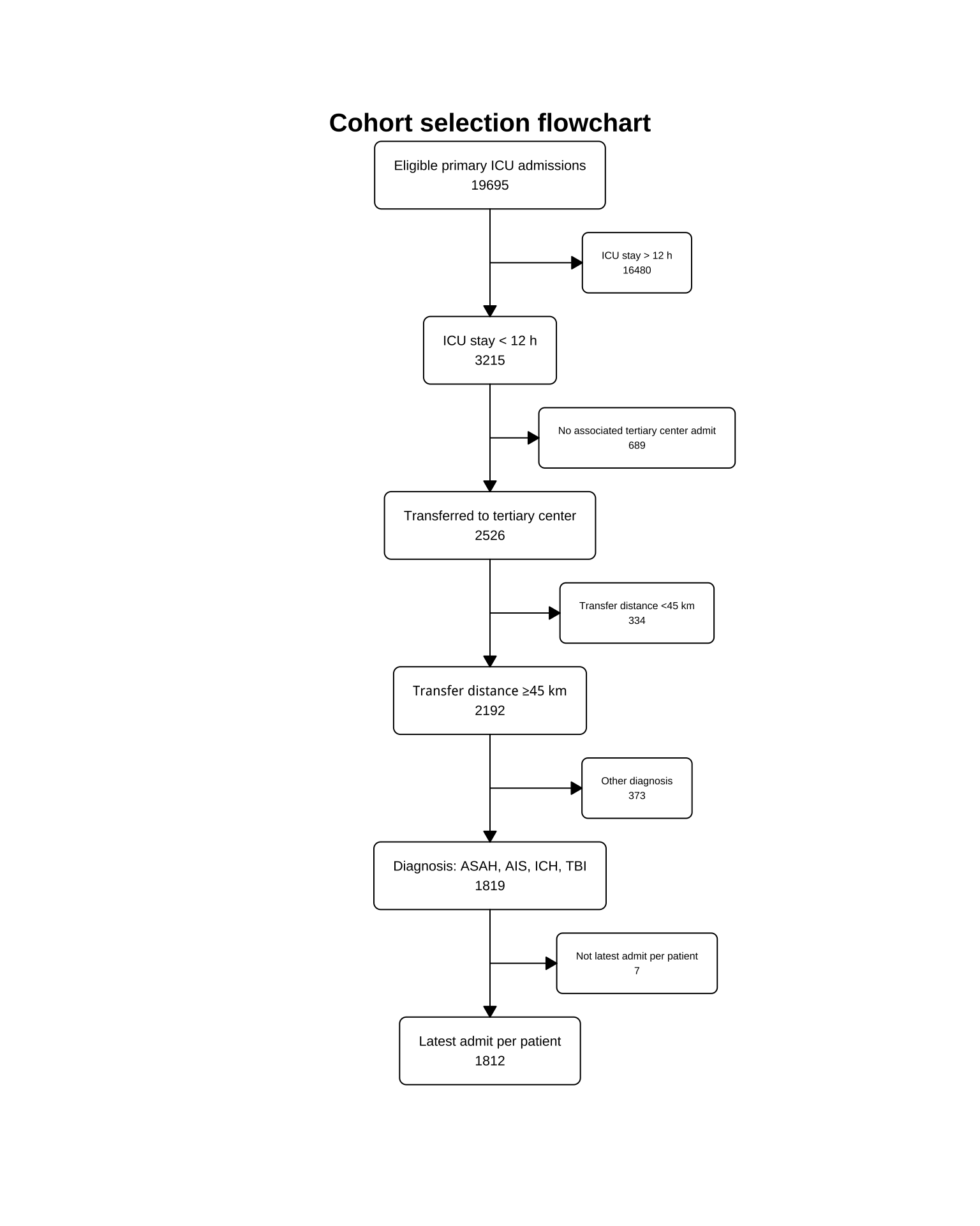
# create patient flowchart
# Start from the full dataset
vtf_ids <- unique(d$VtfId_LopNr)

# Create a tracking dataframe
tracking <- tibble(VtfId_LopNr = vtf_ids)

# Step-by-step filters
d1 <- d %>% filter(sir_dsc_time >= as.Date("2019-10-01") & sir_dsc_time <= as.Date("2024-05-15"))
tracking <- tracking %>%
  mutate(pass_date_range = as.integer(VtfId_LopNr %in% d1$VtfId_LopNr))

d2 <- d1 %>% filter(!is.na(TERTIARY_HADM_ID))
tracking <- tracking %>%
  mutate(pass_tertiary = as.integer(VtfId_LopNr %in% d2$VtfId_LopNr))

d3 <- d2 %>% filter(sir_total_time <= 720)
tracking <- tracking %>%
  mutate(pass_short_icu = as.integer(VtfId_LopNr %in% d3$VtfId_LopNr))

d4 <- d3 %>% filter(SIR_PAR_OFFSET_TIGHT %in% c(-1, 0, 1))
tracking <- tracking %>%
  mutate(pass_recent_par = as.integer(VtfId_LopNr %in% d4$VtfId_LopNr))

d5 <- d4 %>% filter(road_distance >= 45)
tracking <- tracking %>%
  mutate(pass_distance = as.integer(VtfId_LopNr %in% d5$VtfId_LopNr))

d6 <- d5 %>% filter(DX_GROUP %in% c("ASAH", "ICH", "AIS", "TBI"))
tracking <- tracking %>%
  mutate(pass_dx_group = as.integer(VtfId_LopNr %in% d6$VtfId_LopNr))

d7 <- d6 %>%
  group_by(VtfId_LopNr) %>%
  filter(min_rank(DX_RANK) == 1) %>%
  ungroup()
tracking <- tracking %>%
  mutate(pass_dx_rank = as.integer(VtfId_LopNr %in% d7$VtfId_LopNr))

d8 <- d7 %>%
  group_by(LopNr) %>%
  slice_max(sir_dsc_time, n = 1, with_ties = FALSE) %>%
  ungroup()
tracking <- tracking %>%
  mutate(pass_latest_admit = as.integer(VtfId_LopNr %in% d8$VtfId_LopNr))


# Generate flowchart object
d_fc <- tracking %>%
  filter(pass_date_range == 1) %>%
  as_fc(label = "Eligible primary ICU admissions") %>%
  fc_filter(pass_short_icu == 1, label = "ICU stay < 12 h", show_exc = TRUE, label_exc = "ICU stay > 12 h", text_pattern_exc = "{label}\n {n}", text_pattern = "{label}\n {n}") %>%
  fc_filter(pass_tertiary == 1 & pass_recent_par == 1, label = "Transferred to tertiary center", show_exc = TRUE, label_exc = "No associated tertiary center admit", text_pattern_exc = "{label}\n {n}", text_pattern = "{label}\n {n}") %>%
  fc_filter(pass_distance == 1, label = "Transfer distance ≥45 km", show_exc = TRUE, label_exc = "Transfer distance <45 km", text_pattern_exc = "{label}\n {n}", text_pattern = "{label}\n {n}") %>%
  fc_filter(pass_dx_group == 1, label = "Diagnosis: ASAH, AIS, ICH, TBI", show_exc = TRUE, label_exc = "Other diagnosis", text_pattern_exc = "{label}\n {n}", text_pattern = "{label}\n {n}") %>%
  fc_filter(pass_dx_rank == 1 & pass_latest_admit == 1, label = "Latest admit per patient", show_exc = TRUE, label_exc = "Not latest admit per patient", text_pattern_exc = "{label}\n {n}", text_pattern = "{label}\n {n}")
In [8]:
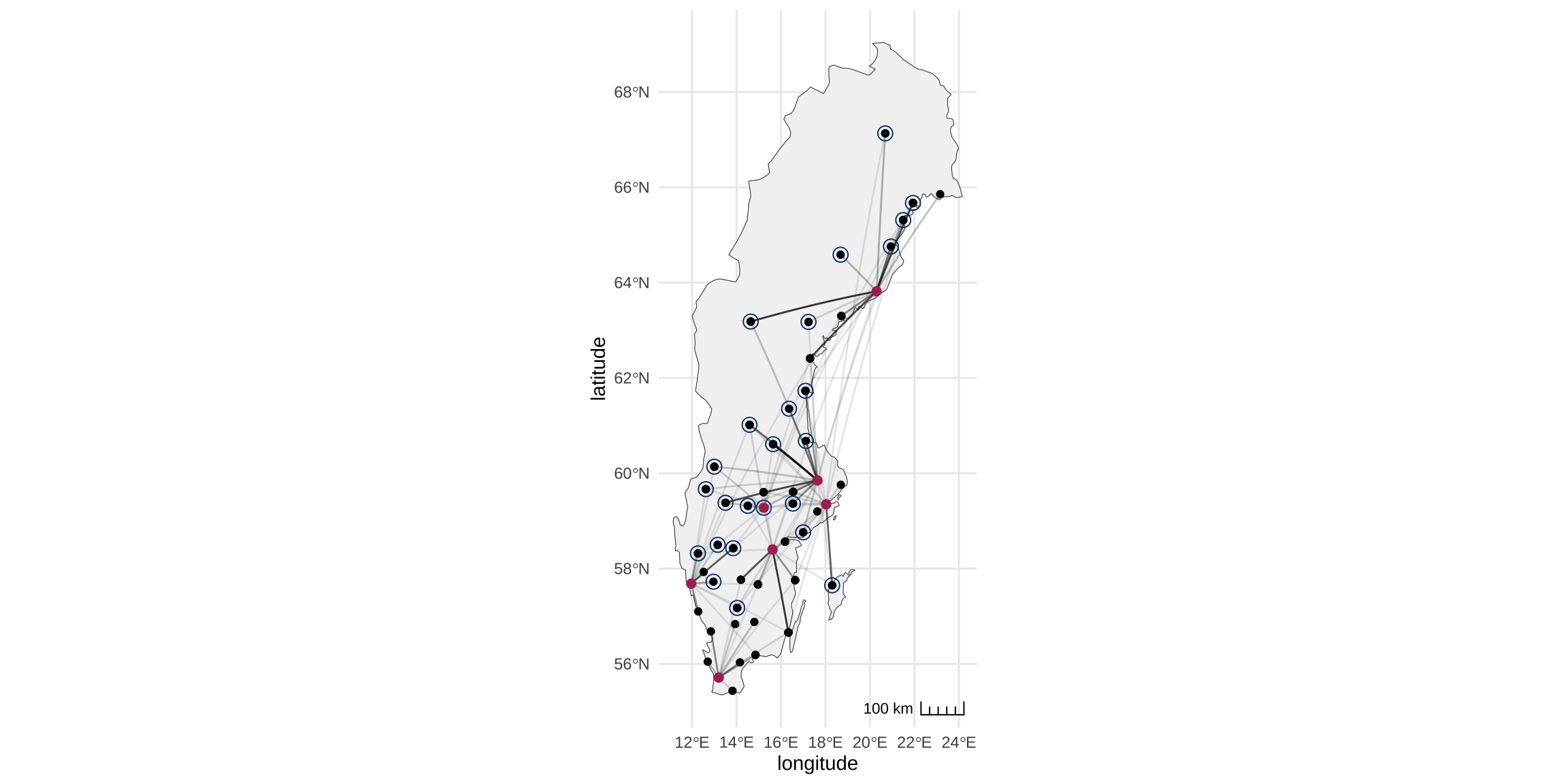
# create map of transfers
library(lwgeom)
Linking to liblwgeom 3.0.0beta1 r16016, GEOS 3.11.0, PROJ 9.1.0
library(ggspatial)
library(geosphere)
library(rnaturalearth)
Warning: package 'rnaturalearth' was built under R version 4.2.3
library(sf)
Warning: package 'sf' was built under R version 4.2.3
Linking to GEOS 3.11.0, GDAL 3.5.3, PROJ 9.1.0; sf_use_s2() is TRUE

Attaching package: 'sf'
The following object is masked from 'package:lwgeom':

    st_perimeter
# Create a dataframe of routes in the dataset and the frequencies
routes <- d_pruned %>%
  group_by(formatted_icu_name, hospital_name_receiving) %>%
  count() %>%
  ungroup() %>%
  arrange(n)

# Create a tibble of longitude and latitude values of sources
sources_tbl <- d_pruned %>% 
  select(start_longitude, start_latitude)
# Create a tibble of longitude and latitude values of destinations
destinations_tbl <- d_pruned %>%
  select(end_longitude, end_latitude)

# Calculate great circles
sl_routes <- gcIntermediate(sources_tbl, destinations_tbl, 
                            n = 50, addStartEnd = TRUE, 
                            sp = TRUE)

# Get mapdata for Sweden from Naturalearth
swe <- ne_countries(scale = "medium", country="Sweden", type="countries", returnclass="sf")

routes_id <- rowid_to_column(routes, var = "id")
routes_long <- routes_id %>% 
  gather(key = "type", value = "place", formatted_icu_name, hospital_name_receiving)

end <- d_pruned %>% select(hospital_name_receiving, end_latitude, end_longitude) %>% rename("place" = "hospital_name_receiving", "latitude" = "end_latitude", "longitude" = "end_longitude")
start <- d_pruned %>% select(formatted_icu_name, start_latitude, start_longitude) %>% rename("place" = "formatted_icu_name", "latitude" = "start_latitude", "longitude" = "start_longitude")
locations <- bind_rows(end, start) %>% distinct()
routes_long_geo <- left_join(routes_long, locations, by = "place")

routes_long_sf <- st_as_sf(routes_long_geo,
                           coords = c("longitude", "latitude"),
                           crs = 4326)

routes_lines <- routes_long_sf %>% 
  group_by(id) %>% 
  summarise(do_union = FALSE) %>% 
  st_cast("LINESTRING")

routes_lines <- left_join(routes_lines, routes_id, by = "id")

routes_sf_tidy <- routes_lines %>% 
  st_segmentize(units::set_units(20, km))

routes_sf_tidy <- routes_lines %>% 
  st_segmentize(units::set_units(20, km))

plot_transfers <- ggplot() +
  geom_sf(data = swe, fill = gray(0.95), color = gray(0.3)) +
  geom_sf(data = routes_sf_tidy, aes(alpha = routes_sf_tidy$n), show.legend = FALSE) +
  scale_alpha_continuous(range = c(0.1, 1), breaks = pretty(range(routes_sf_tidy$n), n = 4)) +
  geom_sf(data = routes_long_sf) +
  geom_point(data = filter(locations, place %in% unique(d_pruned$hospital_name_receiving)), aes(x = longitude, y = latitude), color = "maroon", size = 2) +
  geom_point(shape=21, data = filter(locations, place %in% heavy_users$formatted_icu_name), aes(x = longitude, y = latitude), color = "#004080", size = 3.5) +
  theme_minimal() + 
  ggspatial::annotation_scale(style="ticks", location="br")
In [9]:
# Get palette (manually select better contrast)
clrs <- natparks.pals("Yosemite")
hems_col <- clrs[5]       
non_hems_col <- clrs[20]   
total_col <- "grey30"     # Neutral gray for total bars

# Custom theme using Noto Sans
theme_nice <- function() {
  theme_minimal(base_family = "Noto Sans") +
    theme(
      plot.background = element_rect(fill = "white", color = NA),
      panel.grid.minor = element_blank(),
      panel.grid.major.y = element_line(color = "grey90"),
      plot.title = element_text(face = "bold", size = 16),
      plot.subtitle = element_text(size = 13, margin = margin(b = 10)),
      strip.text = element_text(face = "bold", size = 13),
      strip.background = element_rect(fill = "grey90", color = NA),
      legend.title = element_text(face = "bold", size = 12),
      legend.text = element_text(size = 11),
      axis.text.x = element_text(angle = 45, hjust = 1),
      axis.title.y = element_text(margin = margin(r = 10)),
      plot.margin = margin(10, 15, 10, 15)
    )
}

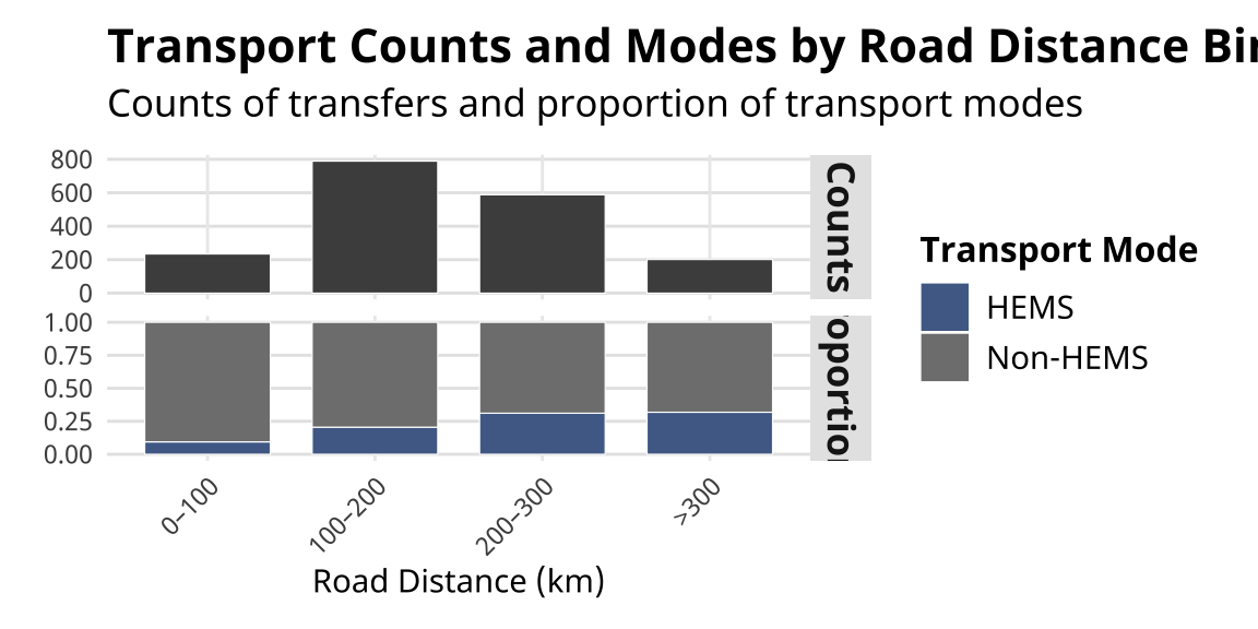
# Define bins
breaks <- c(seq(0, 300, by = 100), Inf)
labels <- c(paste(head(breaks, -2), breaks[-c(1, length(breaks))], sep = "–"), ">300")

# Prepare data
d_plot <- d_pruned %>%
  mutate(
    distance_bin = cut(road_distance, breaks = breaks, labels = labels, right = FALSE),
    distance_bin = factor(distance_bin, levels = labels),
    hems_label = factor(hems_ift, levels = c(TRUE, FALSE), labels = c("HEMS", "Non-HEMS"))
  )

# Count plot
total_counts <- d_plot %>%
  count(distance_bin) %>%
  mutate(
    plot_type = "Counts",
    hems_label = "Total"
  )

# Proportion plot
proportions <- d_plot %>%
  count(distance_bin, hems_label) %>%
  group_by(distance_bin) %>%
  mutate(
    prop = n / sum(n),
    plot_type = "Proportions"
  ) %>%
  ungroup() %>%
  select(distance_bin, hems_label, n = prop, plot_type)

# Combine and fix stacking order
plot_data <- bind_rows(total_counts, proportions) %>%
  mutate(
    hems_label = factor(hems_label, levels = c("Non-HEMS", "HEMS", "Total"))  # HEMS plotted first
  )

# Final plot
transports_bar <- ggplot(plot_data, aes(x = distance_bin, y = n, fill = hems_label)) +
  geom_col(position = "stack", width = 0.75, color = "white", linewidth = 0.2) +
  facet_grid(plot_type ~ ., scales = "free_y") +
  scale_fill_manual(
    values = c(
      "HEMS" = hems_col,
      "Non-HEMS" = non_hems_col,
      "Total" = total_col
    ),
    breaks = c("HEMS", "Non-HEMS")
  ) +
  labs(
    title = "Transport Counts and Modes by Road Distance Bin",
    subtitle = "Counts of transfers and proportion of transport modes",
    x = "Road Distance (km)",
    y = NULL,
    fill = "Transport Mode"
  ) +
  theme_nice()
In [10]:
# Create table with cohort description

cohort_description <- d_pruned %>%
  mutate(hems_ift = case_when(
hems_ift == TRUE ~ "HEMS transfer",
hems_ift == FALSE ~ "Non-HEMS transfer"
  )) %>%
  select(hems_ift, age, sex_female, DX_GROUP, DNR, sir_consciousness_level, SAPS_obtunded, any_AMV, SAPS_total_score, SAPS_score_minus_age_and_gcs, icu_admit_afterhours, icu_admit_nighttime, sir_total_time, road_distance, transit_time_hems, hems_minima_both, daylight, metar_cloud_base, metar_visibility, MORTALITY_30D, MORTALITY_90D, DAOH_90) %>% 
  tbl_summary(by=hems_ift,
              label = list(hems_ift ~ "Interfacility transfer by HEMS",
                           age ~ "Age (years)",
                           sex_female ~ "Female",
                           DX_GROUP ~ "Inferred diagnosis",
                           DNR ~ "DNR order",
                           sir_consciousness_level ~ "SAPS consciousness level",
                           SAPS_obtunded ~ "SAPS GCS <15",
                           any_AMV ~ "Pre-transfer Mechanical Ventilation",
                           SAPS_total_score ~ "SAPS Score",
                           SAPS_score_minus_age_and_gcs ~ "SAPS Score excl. age and GCS components",
                           icu_admit_afterhours ~ "Primary ICU admission outside of office hours",
                           icu_admit_nighttime ~ "Primary ICU admission between 22:00 - 07:00",                     
                           sir_total_time ~ "Time in primary ICU (minutes)",
                           road_distance ~ "Road distance (km)",
                           transit_time_hems ~ "Inferred flight time for HEMS transfers (minutes)",
                           hems_minima_both ~ "HEMS weather minima met at discharge",
                           daylight ~ "Daylight or civil twillight at sending hospital",
                           metar_cloud_base ~ "Cloud base (ft) at sending hospital",
                           metar_visibility ~ "Horizontal visibility (m) at sending hospital",
                           MORTALITY_30D ~ "30-day mortality",
                           MORTALITY_90D ~ "90-day mortality",
                           DAOH_90 ~ "Days alive and out of hospital 90"
                           ),
              statistic = c("transit_time_hems") ~ "{mean}",
              missing_text="Missing"
                        ) %>%
    remove_row_type(variables = c(transit_time_hems, metar_cloud_base, metar_visibility), type = "missing") %>%
    modify_caption(caption = "**Patient characteristics**")
In [11]:
m.modality <- d_pruned %>% 
  mutate(z_SAPS_score_minus_age_and_gcs = scale(SAPS_score_minus_age_and_gcs)) %>%
  mutate(z_age = scale(age)) %>%
    mutate(
    DX_GROUP = forcats::fct_relabel(DX_GROUP, ~ gsub("_", "-", .)),
    sir_consciousness_level = forcats::fct_relabel(sir_consciousness_level, ~ gsub("≤", "le", .))  # or use ASCII-safe levels
  ) %>%
  brm(
  formula = hems_ift ~ DX_GROUP + z_age + SAPS_obtunded + z_SAPS_score_minus_age_and_gcs + icu_admit_nighttime + hems_minima_both + DNR + (1 | formatted_icu_name),
  data = .,
  family = bernoulli(),
  cores = 4,
  chains = 4
)
Warning: Rows containing NAs were excluded from the model.
Compiling Stan program...
Trying to compile a simple C file
Running /Library/Frameworks/R.framework/Resources/bin/R CMD SHLIB foo.c
clang -arch arm64 -I"/Library/Frameworks/R.framework/Resources/include" -DNDEBUG   -I"/Library/Frameworks/R.framework/Versions/4.2-arm64/Resources/library/Rcpp/include/"  -I"/Library/Frameworks/R.framework/Versions/4.2-arm64/Resources/library/RcppEigen/include/"  -I"/Library/Frameworks/R.framework/Versions/4.2-arm64/Resources/library/RcppEigen/include/unsupported"  -I"/Library/Frameworks/R.framework/Versions/4.2-arm64/Resources/library/BH/include" -I"/Library/Frameworks/R.framework/Versions/4.2-arm64/Resources/library/StanHeaders/include/src/"  -I"/Library/Frameworks/R.framework/Versions/4.2-arm64/Resources/library/StanHeaders/include/"  -I"/Library/Frameworks/R.framework/Versions/4.2-arm64/Resources/library/RcppParallel/include/"  -I"/Library/Frameworks/R.framework/Versions/4.2-arm64/Resources/library/rstan/include" -DEIGEN_NO_DEBUG  -DBOOST_DISABLE_ASSERTS  -DBOOST_PENDING_INTEGER_LOG2_HPP  -DSTAN_THREADS  -DUSE_STANC3 -DSTRICT_R_HEADERS  -DBOOST_PHOENIX_NO_VARIADIC_EXPRESSION  -D_HAS_AUTO_PTR_ETC=0  -include '/Library/Frameworks/R.framework/Versions/4.2-arm64/Resources/library/StanHeaders/include/stan/math/prim/fun/Eigen.hpp'  -D_REENTRANT -DRCPP_PARALLEL_USE_TBB=1   -I/opt/R/arm64/include   -fPIC  -falign-functions=64 -Wall -g -O2  -c foo.c -o foo.o
In file included from <built-in>:1:
In file included from /Library/Frameworks/R.framework/Versions/4.2-arm64/Resources/library/StanHeaders/include/stan/math/prim/fun/Eigen.hpp:22:
In file included from /Library/Frameworks/R.framework/Versions/4.2-arm64/Resources/library/RcppEigen/include/Eigen/Dense:1:
In file included from /Library/Frameworks/R.framework/Versions/4.2-arm64/Resources/library/RcppEigen/include/Eigen/Core:19:
/Library/Frameworks/R.framework/Versions/4.2-arm64/Resources/library/RcppEigen/include/Eigen/src/Core/util/Macros.h:679:10: fatal error: 'cmath' file not found
  679 | #include <cmath>
      |          ^~~~~~~
1 error generated.
make: *** [foo.o] Error 1
Start sampling
m.modality.exp_vals <- summary(m.modality)$fixed %>%
  slice(9) %>%
  select("Estimate", "l-95% CI", "u-95% CI") %>%
  unlist() %>%
  exp()
In [12]:
m.modality.summary <- m.modality %>% tbl_regression(exponentiate = TRUE, conf.level = .95,
                              label = c(DX_GROUP ~ "Inferred diagnosis",
                                        icu_admit_nighttime ~ "Primary ICU admission between 22:00 - 07:00",  
                                        SAPS_obtunded ~ "SAPS GCS <15",
                                        DNR ~ "DNR order",
                                        z_age ~ "Age, std",
                                        z_SAPS_score_minus_age_and_gcs ~ "SAPS score (excl. age/GCS components), std",
                                        hems_minima_both ~ "HEMS weather minima met at discharge")
                              ) %>%
  modify_header(estimate = "**aOR**") %>%
  modify_header(label = "**Predictor**") %>%
  modify_caption(caption = "**Multivariate model predicting HEMS transfer**")
Warning in tidy.brmsfit(x, ..., effects = "fixed"): some parameter names
contain underscores: term naming may be unreliable!
In [13]:

m.causal <- d_pruned %>%
  mutate(z_SAPS_score_minus_age_and_gcs = as.numeric(scale(SAPS_score_minus_age_and_gcs))) %>%
  mutate(
    DX_GROUP = forcats::fct_relabel(DX_GROUP, ~ gsub("_", "-", .))
  ) %>%
  mutate(hems_ift = as.integer(hems_ift)) %>%
  mutate(z_age = as.numeric(scale(age))) %>%
 brm(
    formula = MORTALITY_30D ~ hems_ift + (1 + hems_ift | formatted_icu_name) + DX_GROUP + DNR + SAPS_obtunded + z_age + z_SAPS_score_minus_age_and_gcs, 
    data = .,
    family = bernoulli(),
    cores = 4
  )
Warning: Rows containing NAs were excluded from the model.
Compiling Stan program...
Trying to compile a simple C file
Running /Library/Frameworks/R.framework/Resources/bin/R CMD SHLIB foo.c
clang -arch arm64 -I"/Library/Frameworks/R.framework/Resources/include" -DNDEBUG   -I"/Library/Frameworks/R.framework/Versions/4.2-arm64/Resources/library/Rcpp/include/"  -I"/Library/Frameworks/R.framework/Versions/4.2-arm64/Resources/library/RcppEigen/include/"  -I"/Library/Frameworks/R.framework/Versions/4.2-arm64/Resources/library/RcppEigen/include/unsupported"  -I"/Library/Frameworks/R.framework/Versions/4.2-arm64/Resources/library/BH/include" -I"/Library/Frameworks/R.framework/Versions/4.2-arm64/Resources/library/StanHeaders/include/src/"  -I"/Library/Frameworks/R.framework/Versions/4.2-arm64/Resources/library/StanHeaders/include/"  -I"/Library/Frameworks/R.framework/Versions/4.2-arm64/Resources/library/RcppParallel/include/"  -I"/Library/Frameworks/R.framework/Versions/4.2-arm64/Resources/library/rstan/include" -DEIGEN_NO_DEBUG  -DBOOST_DISABLE_ASSERTS  -DBOOST_PENDING_INTEGER_LOG2_HPP  -DSTAN_THREADS  -DUSE_STANC3 -DSTRICT_R_HEADERS  -DBOOST_PHOENIX_NO_VARIADIC_EXPRESSION  -D_HAS_AUTO_PTR_ETC=0  -include '/Library/Frameworks/R.framework/Versions/4.2-arm64/Resources/library/StanHeaders/include/stan/math/prim/fun/Eigen.hpp'  -D_REENTRANT -DRCPP_PARALLEL_USE_TBB=1   -I/opt/R/arm64/include   -fPIC  -falign-functions=64 -Wall -g -O2  -c foo.c -o foo.o
In file included from <built-in>:1:
In file included from /Library/Frameworks/R.framework/Versions/4.2-arm64/Resources/library/StanHeaders/include/stan/math/prim/fun/Eigen.hpp:22:
In file included from /Library/Frameworks/R.framework/Versions/4.2-arm64/Resources/library/RcppEigen/include/Eigen/Dense:1:
In file included from /Library/Frameworks/R.framework/Versions/4.2-arm64/Resources/library/RcppEigen/include/Eigen/Core:19:
/Library/Frameworks/R.framework/Versions/4.2-arm64/Resources/library/RcppEigen/include/Eigen/src/Core/util/Macros.h:679:10: fatal error: 'cmath' file not found
  679 | #include <cmath>
      |          ^~~~~~~
1 error generated.
make: *** [foo.o] Error 1
Start sampling

m.causal.exp_vals <- summary(m.causal)$fixed %>%
  slice(2) %>%
  select("Estimate", "l-95% CI", "u-95% CI") %>%
  unlist() %>%
  exp()
In [14]:
m.causal.w.night <- d_pruned %>%
  mutate(z_SAPS_score_minus_age_and_gcs = as.numeric(scale(SAPS_score_minus_age_and_gcs))) %>%
  mutate(hems_ift = as.integer(hems_ift)) %>%
  mutate(
    DX_GROUP = forcats::fct_relabel(DX_GROUP, ~ gsub("_", "-", .))
  ) %>%
  mutate(z_age = as.numeric(scale(age))) %>%
 brm(
    formula = MORTALITY_30D ~ hems_ift + (1 + hems_ift | formatted_icu_name) + DX_GROUP + DNR + SAPS_obtunded + z_age + z_SAPS_score_minus_age_and_gcs + icu_admit_nighttime,
    data = .,
    family = bernoulli(),
    cores = 4
  )
Warning: Rows containing NAs were excluded from the model.
Compiling Stan program...
Trying to compile a simple C file
Running /Library/Frameworks/R.framework/Resources/bin/R CMD SHLIB foo.c
clang -arch arm64 -I"/Library/Frameworks/R.framework/Resources/include" -DNDEBUG   -I"/Library/Frameworks/R.framework/Versions/4.2-arm64/Resources/library/Rcpp/include/"  -I"/Library/Frameworks/R.framework/Versions/4.2-arm64/Resources/library/RcppEigen/include/"  -I"/Library/Frameworks/R.framework/Versions/4.2-arm64/Resources/library/RcppEigen/include/unsupported"  -I"/Library/Frameworks/R.framework/Versions/4.2-arm64/Resources/library/BH/include" -I"/Library/Frameworks/R.framework/Versions/4.2-arm64/Resources/library/StanHeaders/include/src/"  -I"/Library/Frameworks/R.framework/Versions/4.2-arm64/Resources/library/StanHeaders/include/"  -I"/Library/Frameworks/R.framework/Versions/4.2-arm64/Resources/library/RcppParallel/include/"  -I"/Library/Frameworks/R.framework/Versions/4.2-arm64/Resources/library/rstan/include" -DEIGEN_NO_DEBUG  -DBOOST_DISABLE_ASSERTS  -DBOOST_PENDING_INTEGER_LOG2_HPP  -DSTAN_THREADS  -DUSE_STANC3 -DSTRICT_R_HEADERS  -DBOOST_PHOENIX_NO_VARIADIC_EXPRESSION  -D_HAS_AUTO_PTR_ETC=0  -include '/Library/Frameworks/R.framework/Versions/4.2-arm64/Resources/library/StanHeaders/include/stan/math/prim/fun/Eigen.hpp'  -D_REENTRANT -DRCPP_PARALLEL_USE_TBB=1   -I/opt/R/arm64/include   -fPIC  -falign-functions=64 -Wall -g -O2  -c foo.c -o foo.o
In file included from <built-in>:1:
In file included from /Library/Frameworks/R.framework/Versions/4.2-arm64/Resources/library/StanHeaders/include/stan/math/prim/fun/Eigen.hpp:22:
In file included from /Library/Frameworks/R.framework/Versions/4.2-arm64/Resources/library/RcppEigen/include/Eigen/Dense:1:
In file included from /Library/Frameworks/R.framework/Versions/4.2-arm64/Resources/library/RcppEigen/include/Eigen/Core:19:
/Library/Frameworks/R.framework/Versions/4.2-arm64/Resources/library/RcppEigen/include/Eigen/src/Core/util/Macros.h:679:10: fatal error: 'cmath' file not found
  679 | #include <cmath>
      |          ^~~~~~~
1 error generated.
make: *** [foo.o] Error 1
Start sampling
m.causal.w.night.exp_vals <- summary(m.causal)$fixed %>%
  slice(2) %>%
  select("Estimate", "l-95% CI", "u-95% CI") %>%
  unlist() %>%
  exp()
In [15]:
m.causal.w.night.daoh <- d_pruned %>%
  mutate(z_SAPS_score_minus_age_and_gcs = as.numeric(scale(SAPS_score_minus_age_and_gcs))) %>%
  mutate(hems_ift = as.integer(hems_ift)) %>%
  mutate(
    DX_GROUP = forcats::fct_relabel(DX_GROUP, ~ gsub("_", "-", .))
  ) %>%
  mutate(z_age = as.numeric(scale(age))) %>%
  mutate(DAOH_90 = DAOH_90/90) %>%
 brm(formula =  bf(DAOH_90 ~ hems_ift + (1 | formatted_icu_name) + DX_GROUP + SAPS_obtunded + DNR + z_age + z_SAPS_score_minus_age_and_gcs + icu_admit_nighttime,
     zi ~ hems_ift + (1 | formatted_icu_name) + DX_GROUP + SAPS_obtunded + DNR + z_age +  z_SAPS_score_minus_age_and_gcs + icu_admit_nighttime,
     phi ~ hems_ift + (1 | formatted_icu_name) + DX_GROUP + SAPS_obtunded + DNR + z_age + z_SAPS_score_minus_age_and_gcs + icu_admit_nighttime),
    data = .,
    family = zero_inflated_beta()
  )
Warning: Rows containing NAs were excluded from the model.
Compiling Stan program...
Trying to compile a simple C file
Running /Library/Frameworks/R.framework/Resources/bin/R CMD SHLIB foo.c
clang -arch arm64 -I"/Library/Frameworks/R.framework/Resources/include" -DNDEBUG   -I"/Library/Frameworks/R.framework/Versions/4.2-arm64/Resources/library/Rcpp/include/"  -I"/Library/Frameworks/R.framework/Versions/4.2-arm64/Resources/library/RcppEigen/include/"  -I"/Library/Frameworks/R.framework/Versions/4.2-arm64/Resources/library/RcppEigen/include/unsupported"  -I"/Library/Frameworks/R.framework/Versions/4.2-arm64/Resources/library/BH/include" -I"/Library/Frameworks/R.framework/Versions/4.2-arm64/Resources/library/StanHeaders/include/src/"  -I"/Library/Frameworks/R.framework/Versions/4.2-arm64/Resources/library/StanHeaders/include/"  -I"/Library/Frameworks/R.framework/Versions/4.2-arm64/Resources/library/RcppParallel/include/"  -I"/Library/Frameworks/R.framework/Versions/4.2-arm64/Resources/library/rstan/include" -DEIGEN_NO_DEBUG  -DBOOST_DISABLE_ASSERTS  -DBOOST_PENDING_INTEGER_LOG2_HPP  -DSTAN_THREADS  -DUSE_STANC3 -DSTRICT_R_HEADERS  -DBOOST_PHOENIX_NO_VARIADIC_EXPRESSION  -D_HAS_AUTO_PTR_ETC=0  -include '/Library/Frameworks/R.framework/Versions/4.2-arm64/Resources/library/StanHeaders/include/stan/math/prim/fun/Eigen.hpp'  -D_REENTRANT -DRCPP_PARALLEL_USE_TBB=1   -I/opt/R/arm64/include   -fPIC  -falign-functions=64 -Wall -g -O2  -c foo.c -o foo.o
In file included from <built-in>:1:
In file included from /Library/Frameworks/R.framework/Versions/4.2-arm64/Resources/library/StanHeaders/include/stan/math/prim/fun/Eigen.hpp:22:
In file included from /Library/Frameworks/R.framework/Versions/4.2-arm64/Resources/library/RcppEigen/include/Eigen/Dense:1:
In file included from /Library/Frameworks/R.framework/Versions/4.2-arm64/Resources/library/RcppEigen/include/Eigen/Core:19:
/Library/Frameworks/R.framework/Versions/4.2-arm64/Resources/library/RcppEigen/include/Eigen/src/Core/util/Macros.h:679:10: fatal error: 'cmath' file not found
  679 | #include <cmath>
      |          ^~~~~~~
1 error generated.
make: *** [foo.o] Error 1
Start sampling

SAMPLING FOR MODEL 'anon_model' NOW (CHAIN 1).
Chain 1: 
Chain 1: Gradient evaluation took 0.001136 seconds
Chain 1: 1000 transitions using 10 leapfrog steps per transition would take 11.36 seconds.
Chain 1: Adjust your expectations accordingly!
Chain 1: 
Chain 1: 
Chain 1: Iteration:    1 / 2000 [  0%]  (Warmup)
Chain 1: Iteration:  200 / 2000 [ 10%]  (Warmup)
Chain 1: Iteration:  400 / 2000 [ 20%]  (Warmup)
Chain 1: Iteration:  600 / 2000 [ 30%]  (Warmup)
Chain 1: Iteration:  800 / 2000 [ 40%]  (Warmup)
Chain 1: Iteration: 1000 / 2000 [ 50%]  (Warmup)
Chain 1: Iteration: 1001 / 2000 [ 50%]  (Sampling)
Chain 1: Iteration: 1200 / 2000 [ 60%]  (Sampling)
Chain 1: Iteration: 1400 / 2000 [ 70%]  (Sampling)
Chain 1: Iteration: 1600 / 2000 [ 80%]  (Sampling)
Chain 1: Iteration: 1800 / 2000 [ 90%]  (Sampling)
Chain 1: Iteration: 2000 / 2000 [100%]  (Sampling)
Chain 1: 
Chain 1:  Elapsed Time: 27.446 seconds (Warm-up)
Chain 1:                13.83 seconds (Sampling)
Chain 1:                41.276 seconds (Total)
Chain 1: 

SAMPLING FOR MODEL 'anon_model' NOW (CHAIN 2).
Chain 2: 
Chain 2: Gradient evaluation took 0.000728 seconds
Chain 2: 1000 transitions using 10 leapfrog steps per transition would take 7.28 seconds.
Chain 2: Adjust your expectations accordingly!
Chain 2: 
Chain 2: 
Chain 2: Iteration:    1 / 2000 [  0%]  (Warmup)
Chain 2: Iteration:  200 / 2000 [ 10%]  (Warmup)
Chain 2: Iteration:  400 / 2000 [ 20%]  (Warmup)
Chain 2: Iteration:  600 / 2000 [ 30%]  (Warmup)
Chain 2: Iteration:  800 / 2000 [ 40%]  (Warmup)
Chain 2: Iteration: 1000 / 2000 [ 50%]  (Warmup)
Chain 2: Iteration: 1001 / 2000 [ 50%]  (Sampling)
Chain 2: Iteration: 1200 / 2000 [ 60%]  (Sampling)
Chain 2: Iteration: 1400 / 2000 [ 70%]  (Sampling)
Chain 2: Iteration: 1600 / 2000 [ 80%]  (Sampling)
Chain 2: Iteration: 1800 / 2000 [ 90%]  (Sampling)
Chain 2: Iteration: 2000 / 2000 [100%]  (Sampling)
Chain 2: 
Chain 2:  Elapsed Time: 27.456 seconds (Warm-up)
Chain 2:                22.614 seconds (Sampling)
Chain 2:                50.07 seconds (Total)
Chain 2: 

SAMPLING FOR MODEL 'anon_model' NOW (CHAIN 3).
Chain 3: 
Chain 3: Gradient evaluation took 0.000705 seconds
Chain 3: 1000 transitions using 10 leapfrog steps per transition would take 7.05 seconds.
Chain 3: Adjust your expectations accordingly!
Chain 3: 
Chain 3: 
Chain 3: Iteration:    1 / 2000 [  0%]  (Warmup)
Chain 3: Iteration:  200 / 2000 [ 10%]  (Warmup)
Chain 3: Iteration:  400 / 2000 [ 20%]  (Warmup)
Chain 3: Iteration:  600 / 2000 [ 30%]  (Warmup)
Chain 3: Iteration:  800 / 2000 [ 40%]  (Warmup)
Chain 3: Iteration: 1000 / 2000 [ 50%]  (Warmup)
Chain 3: Iteration: 1001 / 2000 [ 50%]  (Sampling)
Chain 3: Iteration: 1200 / 2000 [ 60%]  (Sampling)
Chain 3: Iteration: 1400 / 2000 [ 70%]  (Sampling)
Chain 3: Iteration: 1600 / 2000 [ 80%]  (Sampling)
Chain 3: Iteration: 1800 / 2000 [ 90%]  (Sampling)
Chain 3: Iteration: 2000 / 2000 [100%]  (Sampling)
Chain 3: 
Chain 3:  Elapsed Time: 28.257 seconds (Warm-up)
Chain 3:                12.049 seconds (Sampling)
Chain 3:                40.306 seconds (Total)
Chain 3: 

SAMPLING FOR MODEL 'anon_model' NOW (CHAIN 4).
Chain 4: 
Chain 4: Gradient evaluation took 0.000713 seconds
Chain 4: 1000 transitions using 10 leapfrog steps per transition would take 7.13 seconds.
Chain 4: Adjust your expectations accordingly!
Chain 4: 
Chain 4: 
Chain 4: Iteration:    1 / 2000 [  0%]  (Warmup)
Chain 4: Iteration:  200 / 2000 [ 10%]  (Warmup)
Chain 4: Iteration:  400 / 2000 [ 20%]  (Warmup)
Chain 4: Iteration:  600 / 2000 [ 30%]  (Warmup)
Chain 4: Iteration:  800 / 2000 [ 40%]  (Warmup)
Chain 4: Iteration: 1000 / 2000 [ 50%]  (Warmup)
Chain 4: Iteration: 1001 / 2000 [ 50%]  (Sampling)
Chain 4: Iteration: 1200 / 2000 [ 60%]  (Sampling)
Chain 4: Iteration: 1400 / 2000 [ 70%]  (Sampling)
Chain 4: Iteration: 1600 / 2000 [ 80%]  (Sampling)
Chain 4: Iteration: 1800 / 2000 [ 90%]  (Sampling)
Chain 4: Iteration: 2000 / 2000 [100%]  (Sampling)
Chain 4: 
Chain 4:  Elapsed Time: 25.999 seconds (Warm-up)
Chain 4:                11.768 seconds (Sampling)
Chain 4:                37.767 seconds (Total)
Chain 4: 
In [16]:
tbl.glm.causal <- m.causal %>% tbl_regression(exponentiate = TRUE, conf.level = .95, label = c(
                                        DX_GROUP ~ "Inferred diagnosis",
                                        z_age ~ "Age, std",
                                        SAPS_obtunded ~ "SAPS GCS <15",
                                        DNR ~ "DNR order",
                                        hems_ift ~ "Interfacility transfer by HEMS",
                                        z_SAPS_score_minus_age_and_gcs ~ "SAPS score (excl. age/GCS components), std")#,
                                      #  any_AMV ~ "Pre-transfer Mechanical Ventilation")
                              ) %>%
  modify_header(estimate = "**aOR**") %>%
  modify_header(label = "**Predictor**")
Warning in tidy.brmsfit(x, ..., effects = "fixed"): some parameter names
contain underscores: term naming may be unreliable!
tbl.glm.causal.w.night <- m.causal.w.night %>% tbl_regression(exponentiate = TRUE, conf.level = .95, label = c(
                                        DX_GROUP ~ "Inferred diagnosis",
                                        icu_admit_nighttime ~ "Primary ICU admission between 22:00 - 07:00",  
                                        z_age ~ "Age, std",
                                        SAPS_obtunded ~ "SAPS GCS <15",
                                        DNR ~ "DNR order",
                                        hems_ift ~ "Interfacility transfer by HEMS",
                                        z_SAPS_score_minus_age_and_gcs ~ "SAPS score (excl. age/GCS components), std")#,
                                       # any_AMV ~ "Pre-transfer Mechanical Ventilation")
                              ) %>%
  modify_header(estimate = "**aOR**") %>%
  modify_header(label = "**Predictor**")
Warning in tidy.brmsfit(x, ..., effects = "fixed"): some parameter names
contain underscores: term naming may be unreliable!
## DAOH model
# Copy the model
model_mean_only <- m.causal.w.night.daoh

# Keep only parameters that start with "b_" and exclude "b_phi_" and "b_zi_"
keep_pars <- names(model_mean_only$fit)[
  grepl("^b_", names(model_mean_only$fit)) &
    !grepl("^b_phi_", names(model_mean_only$fit)) &
    !grepl("^b_zi_", names(model_mean_only$fit))
]

# Drop all other draws from the fit
model_mean_only$fit@sim$samples <- lapply(model_mean_only$fit@sim$samples, function(chain) {
  chain[keep_pars]
})
model_mean_only$fit@sim$pars_oi <- keep_pars
model_mean_only$fit@sim$fnames_oi <- keep_pars

# Also update stanfit param names
model_mean_only$fit@model_pars <- keep_pars
model_mean_only$fit@par_dims <- model_mean_only$fit@par_dims[keep_pars]

# Now pass this stripped model to gtsummary

model_c <- model_mean_only %>%
  tbl_regression(exponentiate = TRUE, conf.level = .95, label = c(
                                        DX_GROUP ~ "Inferred diagnosis",
                                        icu_admit_nighttime ~ "Primary ICU admission between 22:00 - 07:00",  
                                        z_age ~ "Age, std",
                                        SAPS_obtunded ~ "SAPS GCS <15",
                                        DNR ~ "DNR order",
                                        hems_ift ~ "Interfacility transfer by HEMS",
                                        z_SAPS_score_minus_age_and_gcs ~ "SAPS score (excl. age/GCS components), std")#,
                                       # any_AMV ~ "Pre-transfer Mechanical Ventilation")
                              ) %>%
  modify_header(estimate = "**aOR**") %>%
  modify_header(label = "**Predictor**")
Warning in tidy.brmsfit(x, ..., effects = "fixed"): some parameter names
contain underscores: term naming may be unreliable!
glm_table <- tbl_merge(tbls = list(tbl.glm.causal, tbl.glm.causal.w.night, model_c), tab_spanner = c("**Model I**", "**Model II**", "**Model III**")) %>% modify_caption(caption = "**Multivariate models predicting 30-day mortality (I, II) and DAOH-90 (III)**")
In [17]:
# calculate marginal effects
cmp_m.causal <- comparisons(m.causal, variables = "hems_ift", re_formula=NULL)
ci_m.causal <- cmp_m.causal %>% tidy() %>% select(estimate) %>% ci(x=., method="HDI")
est_contrast <- cmp_m.causal %>% tidy() %>% select(estimate)

cmp_m.causal.w.night <- comparisons(m.causal.w.night, variables = "hems_ift", re_formula=NULL)
ci_m.causal.w.night <- cmp_m.causal.w.night %>% tidy() %>% select(estimate) %>% ci(x=., method="HDI")
est_contrast.w.night <- cmp_m.causal.w.night %>% tidy() %>% select(estimate)
In [18]:
# prep a minimal dataset for iv models 

d_pruned_minimal <- d_pruned %>%
  filter(formatted_icu_name %in% heavy_users$formatted_icu_name) %>%
  select(hems_minima_both, hems_ift, MORTALITY_30D, icu_admit_nighttime) %>%
  mutate(hems_minima_both = case_when
          (hems_minima_both == 1 ~ TRUE,
           hems_minima_both == 0 ~ FALSE)) %>%
  mutate(MORTALITY_30D = case_when
          (MORTALITY_30D == 1 ~ TRUE,
           MORTALITY_30D == 0 ~ FALSE
            )) %>%
  drop_na()

n_missing_d_pruned_minimal <- d_pruned %>%
  filter(formatted_icu_name %in% heavy_users$formatted_icu_name) %>%
  summarise(n_missing = sum(is.na(hems_minima_both))) %>%
  pull(n_missing)

# Save anonymized minimal dataset for IV models
write_csv(d_pruned_minimal, "data/minimal_iv_dataset.csv")

# Never-takers: among those assigned to treatment (W == 1), was H == 0?
H0_W1_obs <- as.integer(d_pruned_minimal$hems_ift[d_pruned_minimal$hems_minima_both == 1] == 0)

# Always-takers: among those assigned to control (W == 0), was H == 1?
H1_W0_obs <- as.integer(d_pruned_minimal$hems_ift[d_pruned_minimal$hems_minima_both == 0] == 1)

N_obs <- dim(d_pruned_minimal)[1]
W <- as.integer(d_pruned_minimal$hems_minima_both)
H <- as.integer(d_pruned_minimal$hems_ift)
Y <- as.integer(d_pruned_minimal$MORTALITY_30D)
N <- as.integer(d_pruned_minimal$icu_admit_nighttime)

H0_W1_night <- as.integer(d_pruned_minimal$icu_admit_nighttime[d_pruned_minimal$hems_minima_both == 1])
H1_W0_night <- as.integer(d_pruned_minimal$icu_admit_nighttime[d_pruned_minimal$hems_minima_both == 0])

data_list <- list(
  N_i = nrow(d_pruned_minimal),
  N_obs = as.integer(d_pruned_minimal$icu_admit_nighttime),
  W_obs = as.integer(d_pruned_minimal$hems_minima_both),
  H_obs = as.integer(d_pruned_minimal$hems_ift),
  D_obs = as.integer(d_pruned_minimal$MORTALITY_30D),
  H0_W1_obs = H0_W1_obs,
  H1_W0_obs = H1_W0_obs,
  H0_W1_n = length(H0_W1_obs),
  H1_W0_n = length(H1_W0_obs),
  H0_W1_night = H0_W1_night,
  H1_W0_night = H1_W0_night
)
In [19]:
# fit iv models

model_late <-
  "data {
  int<lower=1> N_i;                         // Total observations
  int<lower=0, upper=1> W_obs[N_i];         // Instrument (W)
  int<lower=0, upper=1> H_obs[N_i];         // Treatment (H)
  int<lower=0, upper=1> D_obs[N_i];         // Outcome (Y)

  int<lower=1> H0_W1_n;                     // Number where W=1
  int<lower=0, upper=1> H0_W1_obs[H0_W1_n]; // Was H=0 in those W=1?

  int<lower=1> H1_W0_n;                     // Number where W=0
  int<lower=0, upper=1> H1_W0_obs[H1_W0_n]; // Was H=1 in those W=0?
}

parameters {
  simplex[3] pi;                            // [NT, C, AT]
  real<lower=0, upper=1> P_T_Z[2];        // P(H | W)
  real<lower=0, upper=1> P_Y_Z[2];        // P(Y | W)
}

model {
  // Priors
  pi ~ dirichlet(rep_vector(0.5, 3));
  for (w in 1:2) {
    P_T_Z[w] ~ beta(0.5, 0.5);
    P_Y_Z[w] ~ beta(0.5, 0.5);
  }

  // Likelihoods
  for (i in 1:N_i) {
    int w = W_obs[i] + 1;

    H_obs[i] ~ bernoulli(P_T_Z[w]);
    D_obs[i] ~ bernoulli(P_Y_Z[w]);
  }

  for (i in 1:H0_W1_n)
    H0_W1_obs[i] ~ bernoulli(pi[1]);  // P(H=0 | W=1): Never-taker

  for (i in 1:H1_W0_n)
    H1_W0_obs[i] ~ bernoulli(pi[3]);  // P(H=1 | W=0): Always-taker
}

generated quantities {
  real LATE;
  real P_H0_W1 = pi[1];
  real P_COMP = pi[2];
  real P_H1_W0 = pi[3];

  LATE = (P_Y_Z[2] - P_Y_Z[1]) / P_COMP;
}"

model_late_conditional <-" 
  data {
  int<lower=1> N_i;                            // Total observations
  int<lower=0, upper=1> W_obs[N_i];            // Instrument (W), 0 or 1
  int<lower=0, upper=1> N_obs[N_i];            // Nighttime indicator (N), 0 or 1
  int<lower=0, upper=1> H_obs[N_i];            // Treatment (H)
  int<lower=0, upper=1> D_obs[N_i];            // Outcome (Y)

  int<lower=1> H0_W1_n;
  int<lower=0, upper=1> H0_W1_obs[H0_W1_n];    // H=0 in W=1 group
  int<lower=0, upper=1> H0_W1_night[H0_W1_n];  // Night indicator for those

  int<lower=1> H1_W0_n;
  int<lower=0, upper=1> H1_W0_obs[H1_W0_n];    // H=1 in W=0 group
  int<lower=0, upper=1> H1_W0_night[H1_W0_n];  // Night indicator for those
}

parameters {
  simplex[3] pi[2];                             // Compliance types [NT, C, AT] by N (0,1)
  real<lower=0, upper=1> P_T_Z[2, 2];           // P(H | W, N) — rows: W=0/1, cols: N=0/1
  real<lower=0, upper=1> P_Y_Z[2, 2];           // P(Y | W, N)
  real<lower=0, upper=1> P_N;                   // P(N = 1) — i.e. nighttime
}

model {
  // Priors
  for (n in 1:2) {
    pi[n] ~ dirichlet(rep_vector(0.5, 3));
  }
  for (w in 1:2) {
    for (n in 1:2) {
      P_T_Z[w, n] ~ beta(0.5, 0.5);
      P_Y_Z[w, n] ~ beta(0.5, 0.5);
    }
  }
  P_N ~ beta(0.5, 0.5);

  // Likelihoods
  for (i in 1:N_i) {
    int w = W_obs[i] + 1;
    int n = N_obs[i] + 1;

    H_obs[i] ~ bernoulli(P_T_Z[w, n]);
    D_obs[i] ~ bernoulli(P_Y_Z[w, n]);
    N_obs[i] ~ bernoulli(P_N);  // This is fine with 0/1
  }

  for (i in 1:H0_W1_n) {
    int n = H0_W1_night[i] + 1;
    H0_W1_obs[i] ~ bernoulli(pi[n][1]);  // NT
  }

  for (i in 1:H1_W0_n) {
    int n = H1_W0_night[i] + 1;
    H1_W0_obs[i] ~ bernoulli(pi[n][3]);  // AT
  }
}

generated quantities {
  vector[2] LATE;
  vector[2] P_H0_W1;
  vector[2] P_COMP;
  vector[2] P_H1_W0;

  for (n in 1:2) {
    P_H0_W1[n] = pi[n][1];
    P_COMP[n] = pi[n][2];
    P_H1_W0[n] = pi[n][3];
    LATE[n] = (P_Y_Z[2, n] - P_Y_Z[1, n]) / P_COMP[n];
  }

  real LATE_marginalized = LATE[2] * P_N + LATE[1] * (1 - P_N);
}
"
In [20]:
# fit iv models
#| 
fit.late <- stan(
  model_code = model_late,
  data = data_list,
  chains = 4,
  iter = 2000,
  seed = 1989
)
Trying to compile a simple C file
Running /Library/Frameworks/R.framework/Resources/bin/R CMD SHLIB foo.c
clang -arch arm64 -I"/Library/Frameworks/R.framework/Resources/include" -DNDEBUG   -I"/Library/Frameworks/R.framework/Versions/4.2-arm64/Resources/library/Rcpp/include/"  -I"/Library/Frameworks/R.framework/Versions/4.2-arm64/Resources/library/RcppEigen/include/"  -I"/Library/Frameworks/R.framework/Versions/4.2-arm64/Resources/library/RcppEigen/include/unsupported"  -I"/Library/Frameworks/R.framework/Versions/4.2-arm64/Resources/library/BH/include" -I"/Library/Frameworks/R.framework/Versions/4.2-arm64/Resources/library/StanHeaders/include/src/"  -I"/Library/Frameworks/R.framework/Versions/4.2-arm64/Resources/library/StanHeaders/include/"  -I"/Library/Frameworks/R.framework/Versions/4.2-arm64/Resources/library/RcppParallel/include/"  -I"/Library/Frameworks/R.framework/Versions/4.2-arm64/Resources/library/rstan/include" -DEIGEN_NO_DEBUG  -DBOOST_DISABLE_ASSERTS  -DBOOST_PENDING_INTEGER_LOG2_HPP  -DSTAN_THREADS  -DUSE_STANC3 -DSTRICT_R_HEADERS  -DBOOST_PHOENIX_NO_VARIADIC_EXPRESSION  -D_HAS_AUTO_PTR_ETC=0  -include '/Library/Frameworks/R.framework/Versions/4.2-arm64/Resources/library/StanHeaders/include/stan/math/prim/fun/Eigen.hpp'  -D_REENTRANT -DRCPP_PARALLEL_USE_TBB=1   -I/opt/R/arm64/include   -fPIC  -falign-functions=64 -Wall -g -O2  -c foo.c -o foo.o
In file included from <built-in>:1:
In file included from /Library/Frameworks/R.framework/Versions/4.2-arm64/Resources/library/StanHeaders/include/stan/math/prim/fun/Eigen.hpp:22:
In file included from /Library/Frameworks/R.framework/Versions/4.2-arm64/Resources/library/RcppEigen/include/Eigen/Dense:1:
In file included from /Library/Frameworks/R.framework/Versions/4.2-arm64/Resources/library/RcppEigen/include/Eigen/Core:19:
/Library/Frameworks/R.framework/Versions/4.2-arm64/Resources/library/RcppEigen/include/Eigen/src/Core/util/Macros.h:679:10: fatal error: 'cmath' file not found
  679 | #include <cmath>
      |          ^~~~~~~
1 error generated.
make: *** [foo.o] Error 1

SAMPLING FOR MODEL 'anon_model' NOW (CHAIN 1).
Chain 1: 
Chain 1: Gradient evaluation took 0.000172 seconds
Chain 1: 1000 transitions using 10 leapfrog steps per transition would take 1.72 seconds.
Chain 1: Adjust your expectations accordingly!
Chain 1: 
Chain 1: 
Chain 1: Iteration:    1 / 2000 [  0%]  (Warmup)
Chain 1: Iteration:  200 / 2000 [ 10%]  (Warmup)
Chain 1: Iteration:  400 / 2000 [ 20%]  (Warmup)
Chain 1: Iteration:  600 / 2000 [ 30%]  (Warmup)
Chain 1: Iteration:  800 / 2000 [ 40%]  (Warmup)
Chain 1: Iteration: 1000 / 2000 [ 50%]  (Warmup)
Chain 1: Iteration: 1001 / 2000 [ 50%]  (Sampling)
Chain 1: Iteration: 1200 / 2000 [ 60%]  (Sampling)
Chain 1: Iteration: 1400 / 2000 [ 70%]  (Sampling)
Chain 1: Iteration: 1600 / 2000 [ 80%]  (Sampling)
Chain 1: Iteration: 1800 / 2000 [ 90%]  (Sampling)
Chain 1: Iteration: 2000 / 2000 [100%]  (Sampling)
Chain 1: 
Chain 1:  Elapsed Time: 0.691 seconds (Warm-up)
Chain 1:                0.649 seconds (Sampling)
Chain 1:                1.34 seconds (Total)
Chain 1: 

SAMPLING FOR MODEL 'anon_model' NOW (CHAIN 2).
Chain 2: 
Chain 2: Gradient evaluation took 8.5e-05 seconds
Chain 2: 1000 transitions using 10 leapfrog steps per transition would take 0.85 seconds.
Chain 2: Adjust your expectations accordingly!
Chain 2: 
Chain 2: 
Chain 2: Iteration:    1 / 2000 [  0%]  (Warmup)
Chain 2: Iteration:  200 / 2000 [ 10%]  (Warmup)
Chain 2: Iteration:  400 / 2000 [ 20%]  (Warmup)
Chain 2: Iteration:  600 / 2000 [ 30%]  (Warmup)
Chain 2: Iteration:  800 / 2000 [ 40%]  (Warmup)
Chain 2: Iteration: 1000 / 2000 [ 50%]  (Warmup)
Chain 2: Iteration: 1001 / 2000 [ 50%]  (Sampling)
Chain 2: Iteration: 1200 / 2000 [ 60%]  (Sampling)
Chain 2: Iteration: 1400 / 2000 [ 70%]  (Sampling)
Chain 2: Iteration: 1600 / 2000 [ 80%]  (Sampling)
Chain 2: Iteration: 1800 / 2000 [ 90%]  (Sampling)
Chain 2: Iteration: 2000 / 2000 [100%]  (Sampling)
Chain 2: 
Chain 2:  Elapsed Time: 0.609 seconds (Warm-up)
Chain 2:                0.617 seconds (Sampling)
Chain 2:                1.226 seconds (Total)
Chain 2: 

SAMPLING FOR MODEL 'anon_model' NOW (CHAIN 3).
Chain 3: 
Chain 3: Gradient evaluation took 8.5e-05 seconds
Chain 3: 1000 transitions using 10 leapfrog steps per transition would take 0.85 seconds.
Chain 3: Adjust your expectations accordingly!
Chain 3: 
Chain 3: 
Chain 3: Iteration:    1 / 2000 [  0%]  (Warmup)
Chain 3: Iteration:  200 / 2000 [ 10%]  (Warmup)
Chain 3: Iteration:  400 / 2000 [ 20%]  (Warmup)
Chain 3: Iteration:  600 / 2000 [ 30%]  (Warmup)
Chain 3: Iteration:  800 / 2000 [ 40%]  (Warmup)
Chain 3: Iteration: 1000 / 2000 [ 50%]  (Warmup)
Chain 3: Iteration: 1001 / 2000 [ 50%]  (Sampling)
Chain 3: Iteration: 1200 / 2000 [ 60%]  (Sampling)
Chain 3: Iteration: 1400 / 2000 [ 70%]  (Sampling)
Chain 3: Iteration: 1600 / 2000 [ 80%]  (Sampling)
Chain 3: Iteration: 1800 / 2000 [ 90%]  (Sampling)
Chain 3: Iteration: 2000 / 2000 [100%]  (Sampling)
Chain 3: 
Chain 3:  Elapsed Time: 0.623 seconds (Warm-up)
Chain 3:                0.565 seconds (Sampling)
Chain 3:                1.188 seconds (Total)
Chain 3: 

SAMPLING FOR MODEL 'anon_model' NOW (CHAIN 4).
Chain 4: 
Chain 4: Gradient evaluation took 8.5e-05 seconds
Chain 4: 1000 transitions using 10 leapfrog steps per transition would take 0.85 seconds.
Chain 4: Adjust your expectations accordingly!
Chain 4: 
Chain 4: 
Chain 4: Iteration:    1 / 2000 [  0%]  (Warmup)
Chain 4: Iteration:  200 / 2000 [ 10%]  (Warmup)
Chain 4: Iteration:  400 / 2000 [ 20%]  (Warmup)
Chain 4: Iteration:  600 / 2000 [ 30%]  (Warmup)
Chain 4: Iteration:  800 / 2000 [ 40%]  (Warmup)
Chain 4: Iteration: 1000 / 2000 [ 50%]  (Warmup)
Chain 4: Iteration: 1001 / 2000 [ 50%]  (Sampling)
Chain 4: Iteration: 1200 / 2000 [ 60%]  (Sampling)
Chain 4: Iteration: 1400 / 2000 [ 70%]  (Sampling)
Chain 4: Iteration: 1600 / 2000 [ 80%]  (Sampling)
Chain 4: Iteration: 1800 / 2000 [ 90%]  (Sampling)
Chain 4: Iteration: 2000 / 2000 [100%]  (Sampling)
Chain 4: 
Chain 4:  Elapsed Time: 0.623 seconds (Warm-up)
Chain 4:                0.737 seconds (Sampling)
Chain 4:                1.36 seconds (Total)
Chain 4: 
fit.late.conditional <- stan(
  model_code = model_late_conditional,
  data = data_list,
  chains = 4,
  iter = 2000,
  seed = 1989
)
Trying to compile a simple C file
Running /Library/Frameworks/R.framework/Resources/bin/R CMD SHLIB foo.c
clang -arch arm64 -I"/Library/Frameworks/R.framework/Resources/include" -DNDEBUG   -I"/Library/Frameworks/R.framework/Versions/4.2-arm64/Resources/library/Rcpp/include/"  -I"/Library/Frameworks/R.framework/Versions/4.2-arm64/Resources/library/RcppEigen/include/"  -I"/Library/Frameworks/R.framework/Versions/4.2-arm64/Resources/library/RcppEigen/include/unsupported"  -I"/Library/Frameworks/R.framework/Versions/4.2-arm64/Resources/library/BH/include" -I"/Library/Frameworks/R.framework/Versions/4.2-arm64/Resources/library/StanHeaders/include/src/"  -I"/Library/Frameworks/R.framework/Versions/4.2-arm64/Resources/library/StanHeaders/include/"  -I"/Library/Frameworks/R.framework/Versions/4.2-arm64/Resources/library/RcppParallel/include/"  -I"/Library/Frameworks/R.framework/Versions/4.2-arm64/Resources/library/rstan/include" -DEIGEN_NO_DEBUG  -DBOOST_DISABLE_ASSERTS  -DBOOST_PENDING_INTEGER_LOG2_HPP  -DSTAN_THREADS  -DUSE_STANC3 -DSTRICT_R_HEADERS  -DBOOST_PHOENIX_NO_VARIADIC_EXPRESSION  -D_HAS_AUTO_PTR_ETC=0  -include '/Library/Frameworks/R.framework/Versions/4.2-arm64/Resources/library/StanHeaders/include/stan/math/prim/fun/Eigen.hpp'  -D_REENTRANT -DRCPP_PARALLEL_USE_TBB=1   -I/opt/R/arm64/include   -fPIC  -falign-functions=64 -Wall -g -O2  -c foo.c -o foo.o
In file included from <built-in>:1:
In file included from /Library/Frameworks/R.framework/Versions/4.2-arm64/Resources/library/StanHeaders/include/stan/math/prim/fun/Eigen.hpp:22:
In file included from /Library/Frameworks/R.framework/Versions/4.2-arm64/Resources/library/RcppEigen/include/Eigen/Dense:1:
In file included from /Library/Frameworks/R.framework/Versions/4.2-arm64/Resources/library/RcppEigen/include/Eigen/Core:19:
/Library/Frameworks/R.framework/Versions/4.2-arm64/Resources/library/RcppEigen/include/Eigen/src/Core/util/Macros.h:679:10: fatal error: 'cmath' file not found
  679 | #include <cmath>
      |          ^~~~~~~
1 error generated.
make: *** [foo.o] Error 1

SAMPLING FOR MODEL 'anon_model' NOW (CHAIN 1).
Chain 1: 
Chain 1: Gradient evaluation took 0.000293 seconds
Chain 1: 1000 transitions using 10 leapfrog steps per transition would take 2.93 seconds.
Chain 1: Adjust your expectations accordingly!
Chain 1: 
Chain 1: 
Chain 1: Iteration:    1 / 2000 [  0%]  (Warmup)
Chain 1: Iteration:  200 / 2000 [ 10%]  (Warmup)
Chain 1: Iteration:  400 / 2000 [ 20%]  (Warmup)
Chain 1: Iteration:  600 / 2000 [ 30%]  (Warmup)
Chain 1: Iteration:  800 / 2000 [ 40%]  (Warmup)
Chain 1: Iteration: 1000 / 2000 [ 50%]  (Warmup)
Chain 1: Iteration: 1001 / 2000 [ 50%]  (Sampling)
Chain 1: Iteration: 1200 / 2000 [ 60%]  (Sampling)
Chain 1: Iteration: 1400 / 2000 [ 70%]  (Sampling)
Chain 1: Iteration: 1600 / 2000 [ 80%]  (Sampling)
Chain 1: Iteration: 1800 / 2000 [ 90%]  (Sampling)
Chain 1: Iteration: 2000 / 2000 [100%]  (Sampling)
Chain 1: 
Chain 1:  Elapsed Time: 1.122 seconds (Warm-up)
Chain 1:                0.917 seconds (Sampling)
Chain 1:                2.039 seconds (Total)
Chain 1: 

SAMPLING FOR MODEL 'anon_model' NOW (CHAIN 2).
Chain 2: 
Chain 2: Gradient evaluation took 0.000117 seconds
Chain 2: 1000 transitions using 10 leapfrog steps per transition would take 1.17 seconds.
Chain 2: Adjust your expectations accordingly!
Chain 2: 
Chain 2: 
Chain 2: Iteration:    1 / 2000 [  0%]  (Warmup)
Chain 2: Iteration:  200 / 2000 [ 10%]  (Warmup)
Chain 2: Iteration:  400 / 2000 [ 20%]  (Warmup)
Chain 2: Iteration:  600 / 2000 [ 30%]  (Warmup)
Chain 2: Iteration:  800 / 2000 [ 40%]  (Warmup)
Chain 2: Iteration: 1000 / 2000 [ 50%]  (Warmup)
Chain 2: Iteration: 1001 / 2000 [ 50%]  (Sampling)
Chain 2: Iteration: 1200 / 2000 [ 60%]  (Sampling)
Chain 2: Iteration: 1400 / 2000 [ 70%]  (Sampling)
Chain 2: Iteration: 1600 / 2000 [ 80%]  (Sampling)
Chain 2: Iteration: 1800 / 2000 [ 90%]  (Sampling)
Chain 2: Iteration: 2000 / 2000 [100%]  (Sampling)
Chain 2: 
Chain 2:  Elapsed Time: 1.099 seconds (Warm-up)
Chain 2:                0.939 seconds (Sampling)
Chain 2:                2.038 seconds (Total)
Chain 2: 

SAMPLING FOR MODEL 'anon_model' NOW (CHAIN 3).
Chain 3: 
Chain 3: Gradient evaluation took 0.000119 seconds
Chain 3: 1000 transitions using 10 leapfrog steps per transition would take 1.19 seconds.
Chain 3: Adjust your expectations accordingly!
Chain 3: 
Chain 3: 
Chain 3: Iteration:    1 / 2000 [  0%]  (Warmup)
Chain 3: Iteration:  200 / 2000 [ 10%]  (Warmup)
Chain 3: Iteration:  400 / 2000 [ 20%]  (Warmup)
Chain 3: Iteration:  600 / 2000 [ 30%]  (Warmup)
Chain 3: Iteration:  800 / 2000 [ 40%]  (Warmup)
Chain 3: Iteration: 1000 / 2000 [ 50%]  (Warmup)
Chain 3: Iteration: 1001 / 2000 [ 50%]  (Sampling)
Chain 3: Iteration: 1200 / 2000 [ 60%]  (Sampling)
Chain 3: Iteration: 1400 / 2000 [ 70%]  (Sampling)
Chain 3: Iteration: 1600 / 2000 [ 80%]  (Sampling)
Chain 3: Iteration: 1800 / 2000 [ 90%]  (Sampling)
Chain 3: Iteration: 2000 / 2000 [100%]  (Sampling)
Chain 3: 
Chain 3:  Elapsed Time: 1.123 seconds (Warm-up)
Chain 3:                0.949 seconds (Sampling)
Chain 3:                2.072 seconds (Total)
Chain 3: 

SAMPLING FOR MODEL 'anon_model' NOW (CHAIN 4).
Chain 4: 
Chain 4: Gradient evaluation took 0.000124 seconds
Chain 4: 1000 transitions using 10 leapfrog steps per transition would take 1.24 seconds.
Chain 4: Adjust your expectations accordingly!
Chain 4: 
Chain 4: 
Chain 4: Iteration:    1 / 2000 [  0%]  (Warmup)
Chain 4: Iteration:  200 / 2000 [ 10%]  (Warmup)
Chain 4: Iteration:  400 / 2000 [ 20%]  (Warmup)
Chain 4: Iteration:  600 / 2000 [ 30%]  (Warmup)
Chain 4: Iteration:  800 / 2000 [ 40%]  (Warmup)
Chain 4: Iteration: 1000 / 2000 [ 50%]  (Warmup)
Chain 4: Iteration: 1001 / 2000 [ 50%]  (Sampling)
Chain 4: Iteration: 1200 / 2000 [ 60%]  (Sampling)
Chain 4: Iteration: 1400 / 2000 [ 70%]  (Sampling)
Chain 4: Iteration: 1600 / 2000 [ 80%]  (Sampling)
Chain 4: Iteration: 1800 / 2000 [ 90%]  (Sampling)
Chain 4: Iteration: 2000 / 2000 [100%]  (Sampling)
Chain 4: 
Chain 4:  Elapsed Time: 1.162 seconds (Warm-up)
Chain 4:                0.951 seconds (Sampling)
Chain 4:                2.113 seconds (Total)
Chain 4: 
# Extract posteriors
posterior.late <- extract(fit.late)
posterior.late <- as.data.frame(rstan::extract(fit.late))

posterior.conditional <- extract(fit.late.conditional)
posterior.late.conditional <- as.data.frame(rstan::extract(fit.late.conditional))
In [21]:
# calc iv bounds
library(ivtools)

iv.b <- ivbounds(data = d_pruned_minimal, Z = "hems_minima_both", X = "hems_ift", Y = "MORTALITY_30D", monotonicity = TRUE)
CRD_lower <- iv.b$p1["min"] - iv.b$p0["max"]
CRD_upper <- iv.b$p1["max"] - iv.b$p0["min"]

Abstract

Background: The optimal transfer team setup and transportation modality in long distance transfers of neuro ICU patients is unknown. The purpose of this study was to estimate the effect of helicopter emergency medical services (HEMS) on 30-day mortality in neuro ICU patients transferred to tertiary centers for definitive care.

Methods: We performed a retrospective cohort study using Swedish healthcare registries and flight movement data. Patients transferred by HEMS were compared to those transferred by other modalities. Observed weather conditions affect flight feasibility were used as a natural randomization mechanism in an instrumental variable analysis.

Results: A total of 1812 patients were transferred from 46 Swedish ICUs. There were 431 HEMS transfers (23.8%). The local average treatment effect of HEMS versus non-HEMS transfer on 30-day mortality was estimated at -3.4% (95% CI: -16.5% to 9.7%). In a risk-adjusted mortality model, the estimated marginal risk difference associated with HEMS was -1.9% (95% CI: -8.2% to 1.8%).

Conclusion: Findings are very weakly suggestive of a potential mortality benefit associated with HEMS transfers. The estimates are limited by statistical uncertainty. Weather minima for HEMS may serve as a useful instrumental variable for causal inference in future observational transport studies.

Introduction

Interfacility transfer is often necessary for critically ill patients with neurological emergencies admitted to community or regional ICUs. In Sweden, as in many other countries, neurosurgical and neurocritical care expertise is centralized to tertiary centers, requiring patients to be transferred for definitive care.

Transporting a critically ill patient between hospitals is challenging. These patients require ongoing treatment and monitoring during transit — ideally at a level at least equivalent to the referring ICU. Environmental factors such as changes in barometric pressure, temperature, and acceleration can exert physiological stress. Operational challenges — limited access to the patient, low lighting, noise, and confined workspace — further complicate care. The transport team must also, concurrent with patient management, solve several non-clinical tasks such as planning the logistics with dispatch centers and communicating with ambulance personnel, receiving providers, and flight crews.

Such challenges may explain the high complication rates observed during interhospital transfers, reported in some studies to affect up to 25% of patients (19). Actual rates may be higher due to reliance on self-reporting (8, 10). Longer transport times are consistently linked to increased complication risk (1, 4, 6).

Some studies suggest that interhospital transfers conducted by specialized retrieval teams may be associated with better care and reduced mortality in adult populations (2, 7, 11, 12). Similar findings have been reported in pediatric cohorts (1316). Only one single-center randomized controlled trial has been conducted to assess the impact of specialized transport teams on patient outcome, which could not establish non-inferiority of nurse led transports (2). Despite the limited evidence base, several expert groups and professional societies recommend that interfacility transfers of critically ill patients be conducted by specialized teams (1720).

However, few studies have specifically examined interhospital transfers of neurocritical care patients, and only one has evaluated the impact of transport modality on outcomes in this population (2123).

In Sweden, two similar patients may be transferred by different means, and under markedly different standards of care. Broadly, there are two provider configurations for interhospital transfers. Specialized retrieval teams — typically composed of an anesthesiologist-intensivist and a nurse trained in anesthesia and/or intensive care — operate at a regional level and have access to both air and ground transport. In contrast, local solutions are based at the referring hospital. These may consist of a single provider, typically a nurse with anesthetic training or a physician in training. Local providers or teams rely solely on ground ambulances. All patients transferred between hospitals via HEMS in Sweden are managed by specialized retrieval teams.

The factors influencing the choice of transport modality in interhospital ICU transfers have not been described. It is possible that estimated transport time, clinical urgency, weather, patient characteristics and local practice patterns play a role in the decision-making process.

In this study, we describe a national cohort of neurocritically ill patients transferred to tertiary centers. We examine predictors of HEMS use and assess whether HEMS — serving in part as a proxy for specialized teams — is associated with 30-day mortality. To strengthen causal inference, we use weather data as an instrumental variable to estimate the effect of transport modality in the presence of potentially uncontrolled confounders, following an assessment of its validity as an instrumental variable.

Methods

Ethics Approval

Ethical approval was granted by the Swedish Ethical Review Authority (Dnr 2022-03054-01, Dnr 2024-00776-02). The manuscript follows the STROBE reporting guidelines for observational studies (24).

Data Sources

Clinical data were obtained from the Swedish Intensive Care Registry (SIR), a national quality registry covering over 80 ICUs, representing most community and regional hospitals in Sweden. SIR includes detailed information on ICU admissions, discharge times, diagnostic categories, interventions, and physiological scores such as SAPS 3 and SOFA.

These data were linked to the National Patient Register (NPR), which contains administrative records, procedure codes, and ICD-coded discharge diagnoses. The NPR has near-complete national coverage and fair diagnostic validity for several acute neurological conditions (25).

Mortality data was retrieved from the National Cause of Death Register (CDR), which includes the date and, when available, the cause of death, with near-complete national coverage.

Additional non-clinical data sources were integrated. Flight movement data were provided by FlightRadar24 AB, Stockholm. Historical weather data were sourced from the Swedish Civil Aviation Administration via Ogimet (www.ogimet.com). Geographic coordinates for hospitals, helipads, and airports — as well as road distances between facilities — were obtained using the openrouteservice.org API (HeiGIT), based on OpenStreetMap data.

Data preprocessing and analysis were performed using SQLite version 3.49.1, R version 4.2.1 (2022-06-23), Python version 3.11, and a set of open source software packages (2631).

Patients and Clinical Data

Patients were eligible if they met the following criteria: (1) admission to a non-tertiary ICU between October 1, 2019, and May 15, 2024; (2) age ≥18 years; (3) a diagnosis indicating need of neurocritical care; and (4) a primary ICU stay shorter than 12 hours.

Because not all tertiary ICUs report to the Swedish Intensive Care Registry (SIR), interhospital transfers were identified via the National Patient Register (NPR). The start date corresponds to the introduction of a new helicopter at a major transport organization, improving flight tracking accuracy. Follow-up on mortality and hospital stays was available through December 31, 2024.

Transfers were defined as admissions to a tertiary center on the same calendar day as discharge from the initial ICU. To account for late-day transitions, we also included tertiary admissions on the day before or after ICU discharge if consistent with a continuous care episode. Long-distance transfers were defined as those exceeding 45 km. Based on an estimated road ambulance speed of 90 km/h and 15 minutes for embarking and disembarking, this threshold implies at least one hour spent outside the safety of an ICU during road transport.

Diagnostic data were sourced from the NPR based on predefined ICD-10 and procedural codes (detailed in candidate-queries/transferred-nsicu-cohort-daoh/transferred-cohort-daoh.sql). Patients with aneurysmal subarachnoid hemorrhage (ASAH), acute ischemic stroke (AIS), intracerebral hemorrhage (ICH), or traumatic brain injury (TBI) — the most common indications for neurocritical care — were included in the cohort.

Physiological data and pre-transfer interventions, were retrieved from the SIR record for the initial ICU stay. Glasgow Coma Scale (GCS) scores reflected pre-sedation consciousness and were taken from SAPS assessments. To avoid strong collinearity in regression models, we also calculated a modified SAPS excluding the age and GCS components.

Do-not-resuscitate (DNR) status was based on SIR records from the initial ICU admission. SIR timestamps were used to classify admissions as occurring outside office-hours (office-hours being defined as Monday to Friday, 08:00–17:00) or during nighttime (22:00–07:00).

Exposure

Helicopter flight movements were parsed from Automatic Dependent Surveillance–Broadcast (ADS-B) data. Details on the flight-matching algorithm and processing steps are provided in Supplement A.

Transfers were classified as carried out by HEMS if a matching flight was identified along the same hospital-to-hospital route, with a departure time within ±120 minutes of the ICU discharge. This window accounts for potential clerical discrepancies in discharge times. See the supplementary material for details.

Instrumental Variable

Automated weather reports (METeorological Aerodrome Reports, METARs) were used to assess whether meteorological conditions met the minimum requirements for HEMS operations, assuming two-pilot crews operating under performance class 1 or 2, in accordance with European Union Aviation Safety Agency (EASA) regulations (32). Code for the weather data parsing algorithm and classification criteria are provided in the Supplement A.

Each hospital was matched to the nearest consistently METAR-reporting airport. Weather conditions were evaluated at both sending and receiving sites at the time of ICU discharge. HEMS was considered technically feasible only if EASA weather minima were met at both locations.

Outcomes

The primary outcome was 30-day mortality following initial ICU admission. The secondary outcome was days alive and out of hospital (DAOH) within 90 days. Mortality data were obtained from the National Cause of Death Register, and hospitalization data from the National Patient Register. For patients who died within each time window, DAOH was set to zero.

Statistical Methods

In the descriptive part of the study, continuous variables were presented as medians with interquartile ranges (IQRs). No univariate hypothesis testing was performed between HEMS and non-HEMS groups to avoid overinterpreting descriptive differences as causal. Transfer routes were visualized using a adapted code from Jesse Sadler (33).

Bayesian modeling with non-informative priors was used. The choice of non-informative priors was based on the limited evidence base in the context of neurointensive care transfers and ICU transfers in Sweden in general. Where applicable, model estimates were reported with 95% credible intervals (CI).

A Bayesian generalized linear model with a Bernoulli likelihood and non-informative priors was used to assess predictors of transport modality. The model included a group-level (“random intercept”) effect for sending ICU and was implemented using the brms package in R. Predictor selection was informed by expert knowledge and data availability.

We examined the relationship between transport modality and patient outcomes using three complementary approaches. First, to describe outcome differences while adjusting for measured confounders, we fit Bayesian generalized linear models. A Bernoulli likelihood was used for 30-day mortality, and a zero-inflated beta likelihood for days alive and out of hospital at 90 days (DAOH-90). The models, implemented in brms, employed partial pooling across sending ICUs, allowing each ICU to have its own intercept and HEMS effect parameter. Covariates were selected based on clinical expertise. Results are presented as odds ratios with 95% CIs and as marginal effects of transport modality.

Second, the local average treatment effect (LATE) was estimated using an instrumental variable (IV) approach, leveraging weather-based HEMS operating minima, per The European Union Aviation Safety Agency (EASA), as a pseudo-randomization mechanism (34, 35). IV analysis allows for causal inference in the presence of unmeasured confounders. LATE estimates the effect of treatment in the “complier” subset of patients—those whose treatment status is influenced by the instrumental variable (35). LATE was estimated using a model implemented in rstan with non-informative Jeffreys priors. A detailed description of the estimand and estimator is provided in the methodological supplement. The rstan code is available in the article notebook available online.

Third, nonparametric Balke-Pearl bounds for the average treatment effect (ATE) were estimated under minimal assumptions using the ivtools package (31, 36).

Identification of LATE requires several assumptions: (1) instrumental variable relevance, (2) exclusion restriction, (3) exchangeability, and (4) monotonicity (3438).

Instrumental variable relevance (assumption 1) was assessed by fitting a generalized linear model with HEMS minima as the sole predictor of transport modality. The estimated odds ratio (OR) was 17.8 (95% CI: 9.7 to 35.2).

However, in subgroups from ICUs that rarely or never use HEMS, the instrumental variable must be weak. Including these patients may introduce bias (38), so they were excluded. The cut-off for low HEMS use was set at <10% of transfers, selected pragmatically in the absence of a validated threshold.

While untestable, the exclusion restriction (assumption 2) is plausible given that weather at ICU discharge is unlikely to affect mortality directly. Further, the assumption can be challenged by instrumental inequalities or by detecting an association between the instrumental variable and outcome in subgroups where the instrumental variable cannot influence exposure (36, 38). In our analysis, the instrumental inequality was not violated. Additionally, in the subgroup of patients from ICUs with low HEMS utilization, the instrumental variable showed no clear association with outcome: the univariate GLM yielded an odds ratio of 0.8 (95% CI: 0.5 to 1.3).

In [22]:
In [23]:

cov_variance_tbl
Patient characterstics given weather conditions
Characteristic Weather minima met, N = 1,4461 Weather minima not met, N = 3621
Age, years 63 (51, 73) 64 (53, 74)
Female 600 (41%) 151 (42%)
Inferred diagnosis

    AIS 211 (15%) 44 (12%)
    ASAH 391 (27%) 102 (28%)
    ICH 289 (20%) 65 (18%)
    TBI 555 (38%) 151 (42%)
SAPS GCS <15 1,059 (74%) 271 (75%)
    Missing 19 3
Pre-transfer Mechanical Ventilation 816 (56%) 218 (60%)
SAPS Score 53 (45, 62) 56 (45, 64)
    Missing 1 0
SAPS Score excl. age and GCS components 41 (36, 48) 43 (36, 49)
    Missing 19 3
Primary ICU admission between 22:00 - 07:00 359 (25%) 127 (35%)
30-day mortality 242 (17%) 68 (19%)
90-day mortality 281 (19%) 81 (22%)
Days alive and out of hospital 90 44 (0, 72) 40 (0, 72)
1 Median (IQR); n (%)

The exchangeability assumption (assumption 3), also known as the no unmeasured confounders condition, cannot be formally tested. One proposed falsification strategy is to assess covariate balance across levels of the instrumental variable (38). As shown in (tbl-cov-balance-iv?), selected covariates appear balanced, with no strong evidence of systematic differences.

Since weather varies diurnally and seasonally, the timing of ICU discharge may influence instrumental variable status. Diurnal variation in ICU strain, staffing, or case mix could in principle affect outcomes through more or less site-specific mechanisms, thereby becoming a potential confounding variable.

A 2018 meta-analysis found no association between nighttime ICU admissions and mortality (39). In our cohort, nighttime admission (22:00–07:00) was associated with lower rates of 30-day mortality: OR 0.7 (95% CI: 0.5 to 0.9). Also, a more recent study reported a lower mortality risk for off-hours ICU admissions (40). Therefore, in sensitivity analyses, we included nighttime admission as a covariate in the regression model and used weather as an instrumental variable conditional on admission time.

The monotonicity assumption (assumption 4) requires that the instrumental variable influences exposure in only one direction (38). In this context, it assumes that poor weather never increases the likelihood of HEMS transfer. This is a reasonable assumption given regulatory and operational constraints, and we consider it satisfied.

In summary, the four core assumptions for identifying the local average treatment effect (LATE) appear to be met in the subcohort of patients treated at ICUs that occasionally use HEMS.

Missing data

Patients with missing relevant variables were excluded prior to statistical modelling. The rate of missingness was low. For the linear models up to 1.4% of patients were excluded due to a missing variable. For the LATE estimation, only 2 of 1107 patients (0.2% ) missing weather data, were excluded.

Code and Data Availability

All code used for data preprocessing and analysis is publicly available (mycode?). A fully anonymized, abbreviated dataset used for the instrumental variable analysis is also archived and accessible (mydata?). (Use Zenodo to create doi when repo is finalized.)

Results

Patient Selection

In [24]:

# Render flowchart
d_fc %>% fc_draw(title = "Cohort selection flowchart")
Flowchart of patient inclusion.

Patient selection is described in (fig-flowchart?). A total of 1812 patients were included in the cohort.

Travel Routes

The paths traveled by patients in the cohort are plotted in (fig-sweden?). The distribution of transport distances and transport modality distribution per distance bin are shown in (fig-barplot?). It can be noted that the proportion of HEMS transfers increase with longer transfer distances, however it is likely that some long distance transfers (>300 km) are carried out by fixed-wing.

In [25]:

plot_transfers
Scale on map varies by more than 10%, scale bar may be inaccurate
Routes travelled by patients in the full cohort by all modes of transport. The opacity of the line denotes the relative number of transfers. Receiving tertiary centers are maroon. Centers where >10% of patients are transferred by HEMS are circled. Note that one of the receiving tertiary centers, Örebro University Hospital, also is also acting as a sending center.
In [26]:

transports_bar
Distribution of transport distances (calculated road distance between sending and receiving center) in the cohort and the proportion of transport modality per distance bin.

Description of the Cohort

In [27]:
In [28]:

cohort_description
Patient characteristics
Characteristic HEMS transfer, N = 4311 Non-HEMS transfer, N = 1,3811
Age (years) 61 (48, 72) 64 (52, 73)
Female 185 (43%) 568 (41%)
Inferred diagnosis

    AIS 70 (16%) 185 (13%)
    ASAH 111 (26%) 382 (28%)
    ICH 87 (20%) 268 (19%)
    TBI 163 (38%) 546 (40%)
DNR order 2 (0.5%) 30 (2.2%)
SAPS consciousness level

    I (GCS ≥13) 205 (48%) 636 (47%)
    II (GCS 7-12) 125 (29%) 385 (28%)
    III (GCS 6) 27 (6.3%) 100 (7.3%)
    IV (GCS 5) 23 (5.4%) 67 (4.9%)
    V (GCS ≤4) 48 (11%) 174 (13%)
    Missing 3 19
SAPS GCS <15 304 (71%) 1,030 (76%)
    Missing 3 19
Pre-transfer Mechanical Ventilation 237 (55%) 801 (58%)
SAPS Score 54 (46, 60) 54 (45, 63)
    Missing 1 0
SAPS Score excl. age and GCS components 41 (37, 46) 42 (36, 48)
    Missing 3 19
Primary ICU admission outside of office hours 304 (71%) 975 (71%)
Primary ICU admission between 22:00 - 07:00 113 (26%) 375 (27%)
Time in primary ICU (minutes) 129 (85, 195) 146 (80, 261)
Road distance (km) 212 (162, 287) 162 (111, 250)
Inferred flight time for HEMS transfers (minutes) 41 NA
HEMS weather minima met at discharge 419 (97%) 1,027 (75%)
    Missing 1 3
Daylight or civil twillight at sending hospital 278 (65%) 746 (54%)
Cloud base (ft) at sending hospital 9,999 (3,850, 9,999) 3,600 (1,000, 9,999)
Horizontal visibility (m) at sending hospital 10,000 (10,000, 10,000) 10,000 (9,999, 10,000)
30-day mortality 61 (14%) 249 (18%)
90-day mortality 73 (17%) 290 (21%)
Days alive and out of hospital 90 41 (0, 71) 44 (0, 72)
1 Median (IQR); n (%); Mean

Minor differences between the HEMS and non-HEMS groups are seen: the HEMS group has a slightly lower median age, fewer DNR orders, and longer transport distances. Overall, the groups appear similar across median and mean values of the presented covariates.

Factors Associated With HEMS Transfer

In [29]:
In [30]:

m.modality.summary
Multivariate model predicting HEMS transfer
Predictor aOR 95% CI1
Inferred diagnosis

    AIS
    ASAH 1.05 0.65, 1.66
    ICH 1.24 0.74, 2.03
    TBI 1.24 0.78, 1.97
Age, std 0.85 0.74, 0.98
SAPS GCS <15 1.17 0.83, 1.67
SAPS score (excl. age/GCS components), std 1.24 1.06, 1.46
Primary ICU admission between 22:00 - 07:00 1.10 0.80, 1.48
HEMS weather minima met at discharge 21.6 11.7, 43.1
DNR order 0.11 0.02, 0.51
1 CI = Credible Interval

In the multivariate predictive model of transfer modality, mainly HEMS minima being met clearly predicted the choice of HEMS (aOR 21.6, 95% CI 11.7 to 43.1), see (tbl-modality-model?). Also, having a DNR order was negatively associated with HEMS transfers.

Risk Adjusted Models of HEMS Transfer vs. 30-day Mortality and DAOH-90

In [31]:
In [32]:
glm_table
Multivariate models predicting 30-day mortality (I, II) and DAOH-90 (III)
Predictor Model I Model II Model III
aOR 95% CI1 aOR 95% CI1 aOR 95% CI1
Interfacility transfer by HEMS 0.81 0.51, 1.22 0.81 0.50, 1.24 0.98 0.85, 1.12
Inferred diagnosis


    AIS
    ASAH 0.43 0.28, 0.65 0.43 0.28, 0.66 0.67 0.56, 0.81
    ICH 0.30 0.19, 0.47 0.30 0.19, 0.47 0.55 0.45, 0.68
    TBI 0.32 0.21, 0.48 0.32 0.21, 0.48 1.02 0.85, 1.23
DNR order 3.64 1.59, 8.69 3.63 1.61, 8.46 1.58 0.89, 2.73
SAPS GCS <15 7.35 4.22, 13.3 7.28 4.18, 13.1 0.52 0.46, 0.59
Age, std 1.69 1.43, 2.00 1.67 1.41, 1.99 0.91 0.86, 0.97
SAPS score (excl. age/GCS components), std 1.67 1.43, 1.94 1.67 1.45, 1.92 0.79 0.74, 0.84
Primary ICU admission between 22:00 - 07:00

0.80 0.58, 1.11 1.15 1.02, 1.30
1 CI = Credible Interval

The adjusted odds ratios of the models are shown in (tbl-glm-outcome?). Models I and II predict 30-day mortality using a bernoulli likelihood without and with, respectively, nighttime admission as a covariate. For model III, which uses a zero-inflated beta likelihood, the odds ratios from the count part of the model represent the multiplicative change in the expected number of days alive and out of hospital (DAOH-90) associated with a one-unit increase in the predictor, holding other variables constant. That is, a value greater than 1 indicates a relative increase in DAOH-90, and a value less than 1 indicates a relative decrease. In (tbl-glm-outcome?), only the completely pooled coefficients (“fixed effects”) are shown for brevity.

The fitted models I and II were used to estimate the effect of HEMS transfer on 30-day mortality, conditional on covariates \(C\), while preserving their empirical distribution. The estimated mean risk difference, \(\mathbb{E}[Y^{H=1, C}] - \mathbb{E}[Y^{H=0,C}]\), was -1.9% (95% CI: -8.2% to 1.8%). The probability of HEMS transfer increasing 30-day mortality was 9.4 %.

In a sensitivity analysis including ICU nighttime admission as an additional covariate, the estimated mean risk difference was -1.9% (95% CI: -8.7% to 1.7%).

Instrumental Variable Analysis

Estimation of the Local Average Treatment Effect (LATE)

The local average treatment effect (LATE) of being transferred by HEMS versus non-HEMS on 30-day mortality was estimated at -3.4% (95% CI: -16.5% to 9.7%).

Estimates of the LATE using weather minima as a conditional instrumental variable (given nighttime ICU admission) did not differ meaningfully: -4.2% (95% CI: -17.8% to 8.7%).

Given the data, model, and assumptions, the posterior probability that HEMS reduces 30-day mortality by at least 2.5 percentage points in the complier group (patients whose transport modality was influenced by weather conditions) is 54%. We propose this threshold as a rough benchmark for a clinically and economically meaningful benefit in typical neuro ICU patients, given the high cost and limited availability of helicopter transfers. The posterior probability that HEMS increases 30-day mortality in the complier group is 31.5%.

Estimation of Bounds on the Average Treatment Effect (ATE)

Balke-Pearl bounds for the risk difference between HEMS and non-HEMS transfers were calculated in the patients send from hospitals that occasionally use HEMS. The lower bound was -14% and the upper bound was 45%

Discussion

Key findings

In a Swedish cohort of neuro ICU patients requiring urgent transfer to a higher level of care, weather minima emerged as the strongest predictor of whether HEMS was utilized. Younger age and higher SAPS scores were also associated with an increased likelihood of HEMS use, whereas the patient having a DNR order placed decresed the likelihood of HEMS transfer.

Both generalized linear models (GLMs), assessing the adjusted association between HEMS transfers and 30-day mortality, and IV analyses estimating the local average treatment effect (LATE), suggest a possible reduction in 30-day mortality associated with HEMS transfers. However, wide uncertainty intervals warrant cautious interpretation.

Findings in Relation to Previous Research

Previous studies examining the association between HEMS interfacility transfers and outcomes have reported mixed findings, with some suggesting benefits and others showing no clear effect (2, 7, 11, 12). Most have been observational in nature and subject to confounders. Our estimates, though imprecise, are consistent with a potential mortality benefit. By using a natural experiment design to help mitigate confounders, this study offers complementary evidence in a field where data from randomized trials remain limited.

Instrumental variable methods remain relatively uncommon in intensive care research. A few notable exceptions have applied parametric two-stage regression models to estimate treatment effects using IVs (4143). These models rely on assumptions about the functional form of the model and the distribution of error terms, which, if violated, can compromise estimates.

The instrumental variables used in those studies include: prior regional HEMS usage (as an instrument for prehospital HEMS vs. ground EMS selection), ICU bed availability (as a proxy for ICU admission promptness), and provider preference (as an instrument for prophylactic magnesium use to prevent atrial fibrillation). All of these IVs are, in effect, variants of region-, hospital-, or provider-level preferences. However, such instruments risk violating the exchangeability assumptions, since they may influence patient outcomes through multiple pathways—not solely through the treatment of interest.

While we commend these studies for advancing causal inference in intensive care research, they also underscore the challenge of identifying valid instrumental variables. In contrast, weather conditions may provide a defensible instrumental variable for studying the effectiveness of HEMS. To our knowledge, this is the first study to use weather minima as an instrumental variable to examine the effect of HEMS interfacility transfers.

Limitations

Patients who die during transfer may be underrepresented, as such patients may not be admitted at the receiving center. Nevertheless, in-transfer deaths are rare in ICU interfacility transfers (1, 9), making substantial bias from this source unlikely.

Another limitation concerns the studied exposure. We believe that the composition of the transfer team, rather than the choice of vehicle, is the key factor influencing patient outcomes. While HEMS transfers serve as a proxy for specialized team involvement, this is an imperfect surrogate. Ground-based transfers may also involve specialized teams, though more commonly they are conducted by local providers. Fixed-wing transfers are performed either by specialized teams or by a single retrieval nurse with anesthetic training. Importantly, transport modality reflects not only team composition but also unmeasured factors such as transit time. Finally, the exposure was inferred from flight records rather than systematically collected clinical data.

In the IV analysis, the estimand was the LATE—reflecting the causal effect among compliers, i.e., patients whose transport modality would vary based on weather minima. The generalizability of this estimate depends on how representative this group is of the broader population and whether effect sizes are consistent across subgroups.

The modest sample size limits precision, particularly given that even optimistic effect sizes would be small (on the order of a few percentage points). Notably, as we moved from GLMs to IV analyses to ATE bounds estimation — each requiring fewer assumptions — uncertainty intervals widened. This reflects the trade-off between statistical certainty and the strength of modeling assumptions (e.g., linearity, homoscedasticity).

Strengths

A key strength of this study is the use of a transparent and reproducible causal inference framework. By leveraging observed weather data to approximate random assignment of transport modality, we strengthen causal inference beyond what is typically achievable with conventional regression methods. Although tailored to our setting, this approach may be applicable in other countries and healthcare systems where HEMS operations are subject to well-defined weather criteria or similar external constraints. In such contexts, comparable methods could support causal inference using observational data to evaluate the effectiveness of HEMS in both interfacility and prehospital care.

Our study integrates high-quality national registry data, which strengthens external validity and supports the generalizability of findings to ICU settings across Sweden.

Implications

The main implications of this study concern both the potential clinical benefit of HEMS and specialized transfer teams in a general neuro ICU population, as well as methodological considerations. Our findings may modestly shift prior beliefs in future studies of interfacility ICU transfer modalities, suggesting a weakly positive effect of HEMS on patient outcomes. Weather minima emerge as a promising instrumental variable for causal inference in both interfacility and prehospital HEMS research, and this approach may be applicable in other healthcare systems. As a secondary observation, we found an unadjusted association between nighttime ICU admission and lower 30-day mortality, which may warrant further investigation.

We propose that weather minima can serve as a valid instrumental variable (IV) for causal inference regarding the effect of HEMS transfers. Where testable, the core IV assumptions appear to be met.

If the LATE estimates reflect a real mortality benefit, practical implications include prioritizing HEMS availability for patients most likely to benefit. This could involve ensuring adequate funding and implementing Point-in-Space (PinS) procedures to expand HEMS operational capacity in poor weather conditions.

Future steps to strengthen inferences about the choice of transfer modality in ICU patients include expanding the cohort to encompass all ICU diagnoses, which—using Swedish registries—could increase the sample to approximately 10,000 patients from 2019 to 2025. Incorporating fixed-wing transport data would help disentangle the effects of team composition from transport mode. Ideally, prospective collection of data on transfer team composition and operational metrics is needed to better characterize the ICU transfer process.

The primary outcome used in this study, 30-day mortality, is relatively coarse. For patients with severe brain injury, functional outcomes are more informative. As a proxy, we included Days Alive and Out of Hospital (DAOH) within 90 days as a secondary outcome. However, prior research shows mixed associations between DAOH and functional outcome (4446). Future studies should preferrably include functional outcomes as an endpoint.

A central principle of neurocritical care is the prevention and management of “secondary insults” — physiological disturbances that exacerbate primary brain injury (47). Hypotension and hypoxia, for example, are such insults that are also commonly reported complications during interfacility transfers (36). Future studies should, in addition to examining transport logistics and team composition, ideally incorporate detailed records of interventions and physiological parameters during transfer. This would enable a better understanding of how care delivery during transport affects patient outcomes and help identify opportunities for improvement. Expanding the Swedish Intensive Care Registry to include data on the transfer process could be a feasible and impactful way to collect a large, generalizable dataset. Since the infrastructure for entering data into the registry is already broadly available, such data gathering could be implemented relatively quickly.

Conclusion

In this national Swedish cohort of emergency interfacility neuro ICU transfers, HEMS weather limitations were the primary determinant of transport modality choice. Findings weakly suggest a potential mortality benefit associated with HEMS but are limited by statistical uncertainty and less-than-ideal outcome granularity. Future prospective studies on transfer modality choice and team composition, using richer data, are needed. HEMS weather minima may offer a useful instrumental variable for causal inference in such work.

List of Abbreviations

ADS-B Automatic Dependent Surveillance–Broadcast

AIS Acute Ischemic Stroke

AMV Assisted Mechanical Ventilation

ASAH Aneurysmal Subarachnoid Hemorrhage

DAOH Days Alive and Out of Hospital

EASA European Union Aviation Safety Agency

GLM Generalized Linear Model

HEMS Helicopter Emergency Medical Services

ICH Intracerebral Hemorrhage

IV Instrumental Variable

LATE Local Average Treatment Effect

METAR Meteorological Aerodrome Report

NPR National Patient Register

SIR Swedish Intensive Care Registry

TBI Traumatic Brain Injury

Funding

Cecilia Åkerlund was supported by Region Stockholm (clinical postdoctoral appointment).

References

1.
Singh JM, MacDonald RD, Bronskill SE, et al.: Incidence and predictors of critical events during urgent air-medical transport [Internet]. Canadian Medical Association Journal 2009; 181:579–584[cited 2023 Nov 15] Available from: http://www.cmaj.ca/cgi/doi/10.1503/cmaj.080886
2.
Van Lieshout EJ, Binnekade J, Reussien E, et al.: Nurses versus physician-led interhospital critical care transport: A randomized non-inferiority trial [Internet]. Intensive Care Medicine 2016; 42:1146–1154[cited 2023 Nov 15] Available from: http://link.springer.com/10.1007/s00134-016-4355-y
3.
Lyphout C, Bergs J, Stockman W, et al.: Patient safety incidents during interhospital transport of patients: A prospective analysis [Internet]. International Emergency Nursing 2018; 36:22–26[cited 2023 Nov 15] Available from: https://linkinghub.elsevier.com/retrieve/pii/S1755599X17300046
4.
Sundbom MF, Sandberg J, Johansson G, et al.: Total Mission Time and Mortality in a Regional Interhospital Critical Care Transport System: A Retrospective Observational Study [Internet]. Air Medical Journal 2021; 40:404–409[cited 2023 Nov 15] Available from: https://linkinghub.elsevier.com/retrieve/pii/S1067991X21001632
5.
Seymour CW, Kahn JM, Schwab CW, et al.: Adverse events during rotary-wing transport of mechanically ventilated patients: A retrospective cohort study [Internet]. Critical Care 2008; 12:R71[cited 2023 Nov 15] Available from: http://ccforum.biomedcentral.com/articles/10.1186/cc6909
6.
Swickard S, Winkelman C, Hustey FM, et al.: Patient Safety Events during Critical Care Transport [Internet]. Air Medical Journal 2018; 37:253–258[cited 2023 Nov 15] Available from: https://linkinghub.elsevier.com/retrieve/pii/S1067991X17303802
7.
Wiegersma JS, Droogh JM, Zijlstra JG, et al.: Quality of interhospital transport of the critically ill: Impact of a Mobile Intensive Care Unit with a specialized retrieval team [Internet]. Critical Care 2011; 15:R75[cited 2023 Nov 15] Available from: http://ccforum.biomedcentral.com/articles/10.1186/cc10064
8.
Grier S, Brant G, Gould TH, et al.: Critical care transfer in an English critical care network: Analysis of 1124 transfers delivered by an ad-hoc system [Internet]. Journal of the Intensive Care Society 2020; 21:33–39[cited 2023 Nov 15] Available from: http://journals.sagepub.com/doi/10.1177/1751143719832175
9.
Jeyaraju M, Andhavarapu S, Palmer J, et al.: Safety Matters: A Meta-analysis of Interhospital Transport Adverse Events in Critically Ill Patients [Internet]. Air Medical Journal 2021; 40:350–358[cited 2023 Nov 15] Available from: https://linkinghub.elsevier.com/retrieve/pii/S1067991X21000882
10.
Archer S, Hull L, Soukup T, et al.: Development of a theoretical framework of factors affecting patient safety incident reporting: A theoretical review of the literature [Internet]. BMJ Open 2017; 7:e017155[cited 2023 Nov 15] Available from: https://bmjopen.bmj.com/lookup/doi/10.1136/bmjopen-2017-017155
11.
Kennedy MP, Gabbe BJ, McKenzie BA: Impact of the introduction of an integrated adult retrieval service on major trauma outcomes [Internet]. Emergency Medicine Journal 2015; 32:833–839[cited 2023 Nov 15] Available from: https://emj.bmj.com/lookup/doi/10.1136/emermed-2014-204376
12.
Bellingan G, Olivier T, Batson S, et al.: Comparison of a specialist retrieval team with current United Kingdom practice for the transport of critically ill patients [Internet]. Intensive Care Medicine 2000; 26:740–744[cited 2023 Nov 15] Available from: http://link.springer.com/10.1007/s001340051241
13.
Ramnarayan P, Thiru K, Parslow RC, et al.: Effect of specialist retrieval teams on outcomes in children admitted to paediatric intensive care units in England and Wales: A retrospective cohort study [Internet]. The Lancet 2010; 376:698–704[cited 2023 Nov 15] Available from: https://linkinghub.elsevier.com/retrieve/pii/S0140673610611130
14.
Orr RA, Felmet KA, Han Y, et al.: Pediatric Specialized Transport Teams Are Associated With Improved Outcomes [Internet]. Pediatrics 2009; 124:40–48[cited 2023 Nov 15] Available from: https://publications.aap.org/pediatrics/article/124/1/40/71705/Pediatric-Specialized-Transport-Teams-Are
15.
Vos GD, Nissen AC, H. M.Nieman F, et al.: Comparison of interhospital pediatric intensive care transport accompanied by a referring specialist or a specialist retrieval team [Internet]. Intensive Care Medicine 2004; 30:302–308[cited 2023 Nov 15] Available from: http://link.springer.com/10.1007/s00134-003-2066-7
16.
Meyer MT, Mikhailov TA, Kuhn EM, et al.: Pediatric Specialty Transport Teams Are Not Associated With Decreased 48-Hour Pediatric Intensive Care Unit Mortality: A Propensity Analysis of the VPS, LLC Database [Internet]. Air Medical Journal 2016; 35:73–78[cited 2023 Nov 15] Available from: https://linkinghub.elsevier.com/retrieve/pii/S1067991X15003284
17.
Droogh JM, Smit M, Absalom AR, et al.: Transferring the critically ill patient: Are we there yet? [Internet]. Critical Care 2015; 19:62[cited 2023 Nov 15] Available from: https://ccforum.biomedcentral.com/articles/10.1186/s13054-015-0749-4
18.
Foëx B, Van Zwanenberg G, Ball J, et al.: Guidance On: The Transfer Of The Critically Ill Adult. 2019;
19.
Warren J, Fromm RE, Orr RA, et al.: Guidelines for the inter- and intrahospital transport of critically ill patients*: [Internet]. Critical Care Medicine 2004; 32:256–262[cited 2023 Nov 15] Available from: http://journals.lww.com/00003246-200401000-00038
20.
Nathanson MH, Andrzejowski J, Dinsmore J, et al.: Guidelines for safe transfer of the brain‐injured patient: Trauma and stroke, 2019: Guidelines from the Association of Anaesthetists and the Neuro Anaesthesia and Critical Care Society [Internet]. Anaesthesia 2020; 75:234–246[cited 2023 Nov 15] Available from: https://associationofanaesthetists-publications.onlinelibrary.wiley.com/doi/10.1111/anae.14866
21.
Safaee MM, Morshed RA, Spatz J, et al.: Interfacility neurosurgical transfers: An analysis of nontraumatic inpatient and emergency department transfers with implications for improvements in care [Internet]. Journal of Neurosurgery 2019; 131:281–289[cited 2024 Aug 9] Available from: https://thejns.org/view/journals/j-neurosurg/131/1/article-p281.xml
22.
Nuño M, Patil CG, Lyden P, et al.: The Effect of Transfer and Hospital Volume in Subarachnoid Hemorrhage Patients [Internet]. Neurocritical Care 2012; 17:312–323[cited 2023 Nov 15] Available from: http://link.springer.com/10.1007/s12028-012-9740-y
23.
Weyhenmeyer J, Guandique CF, Leibold A, et al.: Effects of distance and transport method on intervention and mortality in aneurysmal subarachnoid hemorrhage [Internet]. Journal of Neurosurgery 2018; 128:490–498[cited 2023 Nov 15] Available from: https://thejns.org/view/journals/j-neurosurg/128/2/article-p490.xml
24.
Elm EV, Altman DG, Egger M, et al.: Strengthening the reporting of observational studies in epidemiology (STROBE) statement: Guidelines for reporting observational studies [Internet]. BMJ 2007; 335:806–808[cited 2025 May 1] Available from: https://www.bmj.com/lookup/doi/10.1136/bmj.39335.541782.AD
25.
Köster M, Asplund K, Johansson Å, et al.: Refinement of Swedish Administrative Registers to Monitor Stroke Events on the National Level [Internet]. Neuroepidemiology 2013; 40:240–246[cited 2025 May 1] Available from: https://karger.com/article/doi/10.1159/000345953
26.
Jordahl K, Bossche JVD, Fleischmann M, et al.: Geopandas/geopandas: v0.8.1 [Internet]. 2020; [cited 2025 Jun 11] Available from: https://zenodo.org/record/3946761
27.
Pollard T, Herzman D: Metar.
28.
Team SD: RStan: The R interface to Stan [Internet]. 2025; Available from: https://mc-stan.org/
29.
Bürkner P-C: Brms : An r Package for Bayesian Multilevel Models Using stan [Internet]. Journal of Statistical Software 2017; 80[cited 2025 Jun 11] Available from: http://www.jstatsoft.org/v80/i01/
30.
Sjoberg D D., Whiting K, Curry M, et al.: Reproducible Summary Tables with the gtsummary Package [Internet]. The R Journal 2021; 13:570[cited 2025 Jun 11] Available from: https://journal.r-project.org/archive/2021/RJ-2021-053/index.html
31.
Arvid Sjolander, Elisabeth Dahlqwist, Torben Martinussen: Ivtools: Instrumental Variables [Internet]. 2018; [cited 2025 Jun 11] Available from: https://CRAN.R-project.org/package=ivtools
32.
Regulation (EU) 2023/1020.
33.
Sadler J: Great Circles with R [Internet]. Great Circles with R 2018; Available from: https://www.jessesadler.com/post/great-circles-sp-sf/
34.
Angrist JD, Imbens GW, Rubin DB: Identification of Causal Effects Using Instrumental Variables [Internet]. Journal of the American Statistical Association 1996; 91:444[cited 2025 May 1] Available from: https://www.jstor.org/stable/2291629?origin=crossref
35.
Hernán MA, Robins JM: Causal Inference: What If. Boca Raton: Chapman & Hall/CRC; 2020.
36.
Balke A, Pearl J: Bounds on Treatment Effects from Studies with Imperfect Compliance [Internet]. Journal of the American Statistical Association 1997; 92:1171–1176[cited 2025 May 1] Available from: http://www.tandfonline.com/doi/abs/10.1080/01621459.1997.10474074
37.
Swanson SA, Hernán MA: Commentary: How to Report Instrumental Variable Analyses (Suggestions Welcome) [Internet]. Epidemiology 2013; 24:370–374[cited 2025 May 8] Available from: http://journals.lww.com/00001648-201305000-00007
38.
Labrecque J, Swanson SA: Understanding the Assumptions Underlying Instrumental Variable Analyses: A Brief Review of Falsification Strategies and Related Tools [Internet]. Current Epidemiology Reports 2018; 5:214–220[cited 2025 May 8] Available from: http://link.springer.com/10.1007/s40471-018-0152-1
39.
Galloway M, Hegarty A, McGill S, et al.: The Effect of ICU Out-of-Hours Admission on Mortality: A Systematic Review and Meta-Analysis [Internet]. Critical Care Medicine 2018; 46:290–299[cited 2025 May 10] Available from: https://journals.lww.com/00003246-201802000-00015
40.
Namikata Y, Matsuoka Y, Ito J, et al.: Association between ICU admission during off-hours and in-hospital mortality: A multicenter registry in Japan [Internet]. Journal of Intensive Care 2022; 10:41[cited 2025 May 10] Available from: https://jintensivecare.biomedcentral.com/articles/10.1186/s40560-022-00634-3
41.
Wilson MG, Rashan A, Klapaukh R, et al.: Clinician preference instrumental variable analysis of the effectiveness of magnesium supplementation for atrial fibrillation prophylaxis in critical care [Internet]. Scientific Reports 2022; 12:17433[cited 2025 Jun 13] Available from: https://www.nature.com/articles/s41598-022-21286-1
42.
Harris S, Singer M, Sanderson C, et al.: Impact on mortality of prompt admission to critical care for deteriorating ward patients: An instrumental variable analysis using critical care bed strain [Internet]. Intensive Care Medicine 2018; 44:606–615[cited 2025 Jun 13] Available from: http://link.springer.com/10.1007/s00134-018-5148-2
43.
Tsuchiya A, Tsutsumi Y, Yasunaga H: Outcomes after helicopter versus ground emergency medical services for major trauma–propensity score and instrumental variable analyses: A retrospective nationwide cohort study [Internet]. Scandinavian Journal of Trauma, Resuscitation and Emergency Medicine 2016; 24:140[cited 2025 Jun 13] Available from: http://sjtrem.biomedcentral.com/articles/10.1186/s13049-016-0335-z
44.
Granholm A, Schjørring OL, Jensen AKG, et al.: Association between days alive without life support/out of hospital and health‐related quality of life [Internet]. Acta Anaesthesiologica Scandinavica 2023; 67:762–771[cited 2025 May 18] Available from: https://onlinelibrary.wiley.com/doi/10.1111/aas.14231
45.
Delaney A, Tian DH, Higgins A, et al.: The Association Between Days Alive and Out of Hospital and Health-Related Quality of Life in Patients With Sepsis [Internet]. CHEST Critical Care 2023; 1:100024[cited 2025 May 18] Available from: https://linkinghub.elsevier.com/retrieve/pii/S2949788423000242
46.
Donnelly J, Hong JB, Boyle L, et al.: Days Alive and Out of Hospital as an Outcome Measure in Patients Receiving Hyperacute Stroke Intervention [Internet]. Journal of the American Heart Association 2024; 13:e032321[cited 2025 May 18] Available from: https://www.ahajournals.org/doi/10.1161/JAHA.123.032321
47.
Signorini DF, Andrews PJD, Jones PA, et al.: Adding insult to injury: The prognostic value of early secondary insults for survival after traumatic brain injury [Internet]. Journal of Neurology, Neurosurgery & Psychiatry 1999; 66:26–31[cited 2024 Aug 9] Available from: https://jnnp.bmj.com/lookup/doi/10.1136/jnnp.66.1.26