Local Average Treatment Effect, Estimand and Estimator Explained
As per (1), a LATE estimator can be constructed as follows. Let \(A\) be the treatment, \(Z\) the instrumental variable, and \(Y\) the outcome. All variables are binary. The total population can be divided into four principal strata: always-takers, never-takers, compliers, and defiers. Always-takers are individuals who take the treatment regardless of the instrumental variable. Never-takers are individuals who never take the treatment. Compliers are individuals who take the treatment if the instrumental variable is positive, and do not take it if the instrumental variable is negative. Defiers are individuals who defy the instrumental variable and do the opposite of what it suggests. Given these four principal strata:
Assuming no defiers and an exclusion restriction (i.e., the instrumental variable does not affect the outcome directly), the first, second, and fourth terms vanish. This leaves:
Because compliers adhere to the treatment assigned by the instrumental variable, we can substitute potential outcomes indexed by \(Z\) with those indexed by \(A\):
Solving for the causal effect among compliers yields the LATE estimand:
\[
\mathbb{E}[Y^{a=1} - Y^{a=0} \mid A^{z=1}=1, A^{z=0}=0] =
\frac{\mathbb{E}[Y^{z=1} - Y^{z=0}]}{\Pr(A^{z=1}=1, A^{z=0}=0)}
\] In this study, we use a Bayesian estimator to propagate uncertainty in both the numerator and denominator. We model the outcome \(Y\) as a Bernoulli-distributed random variable conditional on the instrumental variable \(Z\), with a Beta prior placed on the success probabilities:
\[
\Pr(Y \mid Z = z) \sim \mathrm{Beta}(0.5, 0.5)
\]
and
\[
Y_i \sim \mathrm{Bernoulli}(\Pr(Y \mid Z = z_i))
\]
We modeled the population as consisting of three principal strata: never-takers, compliers, and always-takers. The proportions of individuals in each group were denoted by the vector \(\boldsymbol{\pi} = (\pi_{\text{NT}}, \pi_{\text{C}}, \pi_{\text{AT}})\), and assigned a Jeffreys prior:
For subpopulations with empirically identifiable compliance types — those with \(Z = 1, A = 0\) (never-takers) and \(Z = 0, A = 1\) (always-takers) — we included likelihood contributions using Bernoulli observations.
The local average treatment effect (LATE) was estimated as:
\[
\text{LATE} = \frac{\Pr(Y = 1 \mid Z = 1) - \Pr(Y = 1 \mid Z = 0)}{\pi_{\text{C}}}
\]
which corresponds to the average causal effect of treatment among the compliers. Note that the estimator is agebraically equivalent to the Wald estimator since the denominator can be expressed accordingly:
In some settings a population can be broken down into two or more subpopulations. The strength of the instrumental variable (i.e. the proportion of compliers) can differ across such groups. This is also known as first stage heterogeneity, and has recently been highlighted in methodological research.(2, 3)
While a non-zero instrumental variable effect on treatment, the instrumental variable relevance assumption, is necessary for identification of the LATE, it is not necessary for all subgroups.(2, 3) As previously described, the LATE is the average treatment effect (ATE) amongst compliers. Meaning that:
\[
\Pr(\text{LATE}) = \Pr(\text{ATE} \mid \Pi = c)
\] Where \(\Pi = \text{c}\) denotes that the principal strata is complier. According to the law of total probability:
Meaning that the overall LATE is a weighted average of subgroups, where each group is weighted by its contribution to the complier subpopulation.
To describe what happens in the presence of low or zero compliance groups when estimating LATE using the proposed estimator, let there be two subgroups where the first has zero compliance. First, let’s expand the numerator:
\[
\text{LATE} = \frac{\Pr(Y = 1 \mid Z = 1, G = 1) \cdot \Pr(G=1|Z=1) - \Pr(Y = 1 \mid Z = 0, G = 1) \cdot \Pr(G=1|Z=0) + \Pr(Y = 1 \mid Z = 1, G = 2) \cdot \Pr(G=2|Z=1) - \Pr(Y = 1 \mid Z = 0, G = 2) \cdot \Pr(G=2|Z=0) } {\pi_{\text{C}}}
\] Since the instrument, by definition, has no effect on outcome \(Y\) in groups with no compliance we have that
\[
\Pr(Y = 1 \mid Z = 1, G = 1) = \Pr(Y = 1 \mid Z = 0, G = 1) := \tau
\]
And given that group assignment is independent of the instrument (\(Z\mathrel{\bot\mkern-10mu\bot}G\)), we have that
\[
\Pr(G=1|Z=1) = \Pr(G=1|Z=0)
\]
Meaning that only mean zero noise is added to the numerator of the estimator:
\[
\text{LATE} = \frac{
\overbrace{\tau\left[\Pr(G=1 \mid Z=1) - \Pr(G=1 \mid Z=0)\right]}^{\text{mean-zero noise}}
+ \Pr(Y = 1 \mid Z = 1, G = 2) \cdot \Pr(G=2 \mid Z=1)
- \Pr(Y = 1 \mid Z = 0, G = 2) \cdot \Pr(G=2 \mid Z=0)
}{
\pi_{\text{C}}
}
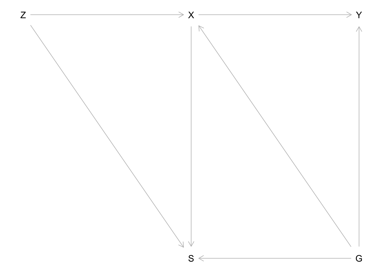
\] Including groups with zero or very low compliance adds noise to the estimator, which may tempt one to exclude such subgroups from the dataset. However, doing so can introduce bias. This can be understood using a graphical approach. Consider a directed acyclic graph (DAG) in which the instrumental variable \(Z\) affects the exposure \(X\), which in turn affects the outcome \(Y\). Introduce a grouping variable \(G\) that may affect both \(X\) and \(Y\). Now define a selection variable \(S\) indicating whether an individual belongs to a low-compliance subgroup by some arbitrary definition. If we condition on \(S\)—for example, by restricting the analysis to high-compliance groups based on \(Z\), \(X\), and \(G\)—we are effectively conditioning on a collider. This opens a non-causal path in the DAG, leading to biased causal estimates. In practice, such “naive” selection produces bias that, in expectation, shrinks estimated causal effects toward zero (2–4).
In [1]:
library(dagitty)
Warning: package 'dagitty' was built under R version 4.2.3
Hazard Y, Löwe S: Improving LATEEstimation in Experiments with ImperfectCompliance.
4.
Canan C, Lesko C, Lau B: Instrumental VariableAnalyses and SelectionBias: [Internet]. Epidemiology 2017; 28:396–398[cited 2025 Aug 10] Available from: http://journals.lww.com/00001648-201705000-00014